2.4 - Guinea pig tooth growth One-Way ANOVA example
by
A second example of the One-way ANOVA methods involves a study of growth rates of the teeth of Guinea Pigs (measured in millimeters, mm). N=60 Guinea Pigs were obtained from a local breeder and each received Orange Juice (OJ) or ascorbic acid (the stuff in vitamin C capsules, called VC below) at one of three dosages (0.5, 1, or 2 mg) as a source of added Vitamin C in their diets. Each guinea pig was randomly assigned to receive one of the six different treatment combinations possible (OJ at 0.5 mg, OJ at 1 mg, OJ at 2 mg, VC at 0.5 mg, VC at 1 mg, and VC at 2 mg). The animals were treated similarly otherwise and we can assume lived in separate cages. We need to create a variable that combines the levels of delivery type (OJ, VC) and the dosages (0.5, 1, and 2) to use our One-Way ANOVA on the six levels. The interaction function creates a new variable in the ToothGrowth data.frame that we called Treat that will be used as a six-level grouping variable.
> data(ToothGrowth) #Available in Base R package
> ToothGrowth$Treat=with(ToothGrowth,interaction(supp,dose)) #Creates a new variable Treat with 6 levels
The tally function helps us to check for balance; this is a balanced design because the same number of guinea pigs (nj=10 for all j) were measured in each treatment combination.
> require(mosaic)
> tally(~Treat,data=ToothGrowth)
| OJ.0.5 | VC.0.5 | OJ.1 | VC.1 | OJ.2 | VC.2 |
| 10 | 10 | 10 | 10 | 10 | 10 |
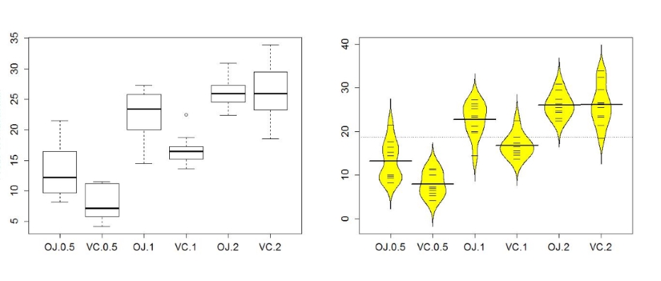
The next task is to visualize the results using boxplots and beanplots27 (Figure 2-14) and generate some summary statistics for each group using favstats.
> par(mfrow=c(1,2))
> boxplot(len~Treat,data=ToothGrowth,ylab="Tooth Growth in mm")
> beanplot(len~Treat,data=ToothGrowth,log="",col="yellow",method="jitter")
> favstats(len~Treat,data=ToothGrowth)
| .group | min | Q1 | median | Q3 | max | mean | sd | n | missing | |
| 1 | OJ.0.5 | 8.2 | 9.700 | 12.25 | 16.175 | 21.5 | 13.23 | 4.459709 | 10 | 0 |
| 2 | VC.0.5 | 4.2 | 5.950 | 7.15 | 10.900 | 11.5 | 7.98 | 2.746634 | 10 | 0 |
| 3 | OJ.1 | 14.5 | 20.300 | 23.45 | 25.650 | 27.3 | 22.70 | 3.910953 | 10 | 0 |
| 4 | VC.1 | 13.6 | 15.275 | 16.50 | 17.300 | 22.5 | 16.77 | 2.515309 | 10 | 0 |
| 5 | OJ.2 | 22.4 | 24.575 | 25.95 | 27.075 | 30.9 | 26.06 | 2.655058 | 10 | 0 |
| 6 | VC.2 | 18.5 | 23.375 | 25.95 | 28.800 | 33.9 | 26.14 | 4.797731 | 10 | 0 |
Figure 2-14 suggests that the mean tooth growth increases with the dosage level and that OJ might lead to higher growth rates than VC except at dosages of 2 mg. The variability around the means looks to be small relative to the differences among the means, so we should expect a small p-value from our F-test. The design is balanced as noted above (nj = 10 for all six groups) so the methods are somewhat resistant to impacts from non-normality and non-constant variance. There is some suggestion of non-constant variance in the plots but this will be explored further below when we can visually remove the difference in the means from this comparison. There might be some skew in the responses in some of the groups but there are only 10 observations per group so skew in the boxplots could be generated by very few observations.
Now we can apply our 6+ steps for performing a hypothesis test with these observations. The initial step is deciding on the claim to be assessed and the test statistic to use. This is a six group situation with a quantitative response, identifying it as a One-Way ANOVA where we want to test a null hypothesis that all the groups have the same population mean. We will use a 5% significance level.
- • The null hypothesis could also be written in reference-coding as H0: τVC0.5 = τOJ1 = τVC1 = τOJ2 = τVC2 = 0 since OJ.0.5 is chosen as the baseline group (discussed below).
- • The alternative hypothesis can be left a bit less specific: HA: Not all τj equal 0.
- • Independence:
- ○ This is where the separate cages note above is important. Suppose that there were cages that contained multiple animals and they competed for food or could share illness. The animals in one cage might be systematically different from the others and this "clustering" of observations would present a potential violation of the independence assumption. If the experiment had the animals in separate cages, there is no clear dependency in the design of the study and can assume that there is no problem with this assumption.
- • Constant variance:
- ○ As noted above, there is some indication of a difference in the variability among the groups in the boxplots but the sample size was small in each group. We need to fit the linear model to get the other diagnostic plots to make an overall assessment.
> m2=lm(len~Treat,data=ToothGrowth)
> par(mfrow=c(2,2))
> plot(m2)

- ○ The Residuals vs Fitted panel in Figure 2-15 shows some difference in the spreads but the spread is not that different between the groups.
- ○ The Scale-Location plot also shows just a little less variability in the group with the smallest fitted value but the spread of the groups looks fairly similar in this alternative scaling.
- ○ Put together, the evidence for non-constant is not that strong and we can assume that there is at least not a major problem with this assumption.
- • Normality of residuals:
- ○ The Normal Q-Q plot shows a small deviation in the lower tail but nothing that we wouldn't expect from a normal distribution. There is no evidence of a problem with this assumption in the upper right panel of Figure 2-15.
- • The ANOVA table for our model follows, providing an F-statistic of 41.557:
> anova(m2)
Analysis of Variance Table
| Response: len | ||||||
| Df | Sum Sq | Mean Sq | F value | Pr(>F) | ||
| Treat | 5 | 2740.10 | 548.02 | 41.557 | < 2.2e-16 | *** |
| Residuals | 54 | 712.11 | 13.19 |
- • There are two options here, especially since it seems that our assumptions about variance and normality are not violated (note that we do not say "met" - we just have no strong evidence against them). The parametric and nonparametric approaches should provide similar results here.
- • The parametric approach is easiest - the p-value comes from the previous ANOVA table as <2.2e-16. This is in scientific notation and means it is at the numerical precision of the computer and it reports that this is a very small number. You report that the p-value<0.00001 but should not report that it is 0. This p-value came from an F(5,54) distribution (the distribution of the test statistic if the null hypothesis is true).
- • The nonparametric approach is not too hard so we can compare the two approaches here.
> Tobs <- anova(lm(len~Treat,data=ToothGrowth))[1,4]; Tobs
[1] 41.55718
> par(mfrow=c(1,2))
> B<- 1000
> Tstar<-matrix(NA,nrow=B)
> for (b in (1:B)){
+ Tstar[b]<-anova(lm(len~shuffle(Treat),data=ToothGrowth))[1,4]
+ }
> hist(Tstar,xlim=c(0,Tobs+3))
> abline(v=Tobs,col="red",lwd=3)
> plot(density(Tstar),,xlim=c(0,Tobs+3),main="Density curve of Tstar")
> abline(v=Tobs,col="red",lwd=3)
> pdata(Tobs,Tstar,lower.tail=F)
[1] 0
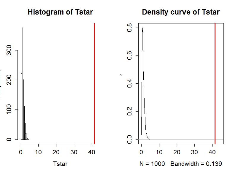
- • The permutation p-value was reported as 0. This should be reported as p-value<0.0001 since we did 1000 permutations and found that none of the permuted F-statistics, F*, were larger than the observed F-statistic of 41.56. The permuted results do not exceed 6 as seen in Figure 2-16, so the observed result is really unusual relative to the null hypothesis. As suggested previously, the parametric and nonparametric approaches should be similar here and they were.
- • Reject H0 since the p-value is less than 5%.
- • There is evidence at the 5% significance level that the different treatments (combinations of OJ/VC and dosage levels) cause some difference in the true mean tooth growth for these Guinea Pigs.
- ○ We can make the causal statement because the treatments were randomly assigned but these inferences only apply to these Guinea Pigs since they were not randomly selected from a larger population.
- ○ Remember that we are making inferences to the population means and not the sample means and want to make that clear in any conclusion.
- ○ The alternative is that there is some difference in the true means - be sure to make the wording clear that you aren't saying that all differ. In fact, if you look back at Figure 2-14, the means for the 2 mg dosages look almost the same. The F-test is about finding evidence of some difference somewhere among the true means. The next section will provide some additional tools to get more specific about the source of those detected differences.
Before we leave this example, we should revisit our model estimates and interpretations. The default model parameterization is into the reference-coding. Running the model summary function on m2 provides the estimated coefficients:
> summary(m2)
Coefficients:
| Estimate Std. | Error | t value | Pr(>|t|) | ||
| (Intercept) | 13.230 | 1.148 | 11.521 | 3.60e-16 | *** |
| TreatVC.0.5 | -5.250 | 1.624 | -3.233 | 0.00209 | ** |
| TreatOJ.1 | 9.470 | 1.624 | 5.831 | 3.18e-07 | *** |
| TreatVC.1 | 3.540 | 1.624 | 2.180 | 0.03365 | * |
| TreatOJ.2 | 12.830 | 1.624 | 7.900 | 1.43e-10 | *** |
| TreatVC.2 | 12.910 | 1.624 | 7.949 | 1.19e-10 | *** |
For some practice with the reference coding used in these models, we will find the estimates for observations for a couple of the groups. To work with the parameters, you need to start with diagnosing the baseline category by considering which level is not displayed in the output. The levels function can list the groups and their coding in the data set. The first level is usually the baseline category but you should check this in the model summary as well.
> levels(ToothGrowth$Treat)
| [1] | "OJ.0.5" | "VC.0.5" | "OJ.1" | "VC.1" | "OJ.2" | "VC.2" |
There is a VC.0.5 in the second row of the model summary, but there is no row for 0J.0.5 and so this must be the baseline category. That means that the fitted value or model estimate for the OJ at 0.5 mg group is the same as the (Intercept) row or α̂, estimating a mean tooth growth of 13.23 mm when the pigs get OJ at a 0.5 mg dosage level. You should always start with working on the baseline level in a reference-coded model. To get estimates for any other group, then you can use the (Intercept) estimate and add the deviation for the group of interest. For VC.0.5, the estimated mean tooth growth is α̂ + τ̂2 = α̂ + τ̂VC.0.5 =13.23+ (-5.25) = 7.98 mm. It is also potentially interesting to directly interpret the estimated difference (or deviation) between OJ0.5 (the baseline) and VC0.5 (group 2) that is τ̂VC.0.5 = -5.25: we estimate that the mean tooth growth in VC.0.5 is 5.25 mm shorter than it is in OJ.0.5. This and many other direct comparisons of groups are likely of interest to researchers involved in studying the impacts of these supplements on tooth growth and the next section will show us how to do that (correctly!).
27Note that to see all the group labels in the plot when I copied it into R, I had to widen the plot window. You can resize the plot window using the small "=" signs in the grey bars that separate the different panels in R-studio.