1.7 - Confidence intervals and bootstrapping
by
Randomly shuffling the treatments between the observations is like randomly sampling the treatments without replacement. In other words, we randomly sample one observation at a time from the treatments until we have n observations. This provides us with a technique for testing hypotheses because it provides a new ordering of the observations that is valid if the null hypothesis is assumed true. In most situations, we also want to estimate parameters of interest and provide confidence intervals for those parameters (an interval where we are __% confident that the true parameter lies). As before, there are two options we will consider - a parametric and a nonparametric approach. The nonparametric approach will be using what is called bootstrapping and draws its name from "pull yourself up by your bootstraps" where you improve your situation based on your own efforts. In statistics, we make our situation or inferences better by re-using the observations we have by assuming that the sample represents the population. Since each observation represents other similar observations in the population, if we sample with replacement from our data set it mimics the process of taking repeated random samples from our population of interest. This process ends up giving us good distributions of statistics even when our standard normality assumption is violated, similar to what we encountered in the permutation tests. Bootstrapping is especially useful in situations where we are interested in statistics other than the mean (say we want a confidence interval for a median or a standard deviation) or when we consider functions of more than one parameter and don't want to derive the distribution of the statistic (say the difference in two medians). Our uses for bootstrapping will be typically to use it when some of our assumptions (especially normality) might be violated for our regular procedure to provide more trustworthy inferences.
To perform bootstrapping, we will use the resample function from the mosaic package. We can apply this function to a data set and get a new version of the data set by sampling new observations with replacement from the original one. The new version of the data set contains a new variable called orig.ids which is the number of the subject from the original data set. By summarizing how often each of these id's occurred in a bootstrapped data set, we can see how the re-sampling works. The code is complicated for unimportant reasons, but the end result is the table function providing counts of the number of times each original observation occurred, with the first row containing the observation number and the second row the count. In the first bootstrap sample shown, the 1st, 2nd, and 4th observations were sampled one time each and the 3rd observation was not sampled at all. The 5th observation was sampled two times. Observation 42 was sampled four times. This helps you understand what types of samples that sampling with replacement can generate.
> table(as.numeric(resample(MockJury2)$orig.ids))
| 1 | 2 | 4 | 5 | 6 | 7 | 8 | 9 | 10 | 11 | 12 | 14 | 15 | 17 | 23 | 24 | 25 | 26 | 27 | 28 | 32 | 33 | 35 | 36 | 37 |
| 1 | 1 | 1 | 2 | 1 | 1 | 1 | 1 | 2 | 1 | 1 | 1 | 1 | 2 | 2 | 1 | 2 | 1 | 2 | 1 | 2 | 3 | 1 | 2 | 3 |
| 39 | 41 | 42 | 43 | 44 | 45 | 47 | 51 | 54 | 56 | 57 | 58 | 59 | 60 | 61 | 62 | 63 | 65 | 66 | 68 | 70 | 71 | 73 | 75 | |
| 1 | 2 | 4 | 2 | 1 | 1 | 1 | 2 | 1 | 1 | 1 | 1 | 2 | 1 | 1 | 2 | 1 | 2 | 1 | 1 | 2 | 2 | 2 | 3 |
A second bootstrap sample is also provided. It did not re-sample observations 1, 2, or 4 but does sample observation 5 three times. You can see other variations in the resulting re-sampling of subjects.
> table(as.numeric(resample(MockJury2)$orig.ids))
| 3 | 5 | 6 | 8 | 10 | 12 | 15 | 16 | 17 | 18 | 19 | 25 | 26 | 27 | 29 | 30 | 32 | 34 | 36 | 37 | 38 | 39 | 40 | 4 | 42 |
| 1 | 3 | 1 | 2 | 1 | 1 | 1 | 1 | 2 | 1 | 1 | 3 | 1 | 1 | 1 | 1 | 2 | 2 | 1 | 2 | 2 | 1 | 2 | 1 | 2 |
| 44 | 45 | 47 | 48 | 49 | 52 | 53 | 55 | 56 | 57 | 58 | 60 | 61 | 63 | 64 | 65 | 66 | 67 | 68 | 69 | 70 | 71 | 72 | 73 | 74 |
| 2 | 1 | 1 | 1 | 3 | 1 | 1 | 1 | 1 | 1 | 3 | 1 | 1 | 3 | 2 | 1 | 1 | 2 | 1 | 1 | 1 | 1 | 2 | 2 | 2 |
| 75 | ||||||||||||||||||||||||
| 1 |
Each run of the resample function provides a new version of the data set. Repeating this B times using another for loop, we will track our quantity of interest, say T, in all these new "data sets" and call those results T*. The distribution of the bootstrapped T* statistics will tell us about the range of results to expect for the statistic and the middle __% of the T*'s provides a bootstrap confidence interval for the true parameter - here the difference in the two population means.
To make this concrete, we can revisit our previous examples, starting with the MockJury2 data created before and our interest in comparing the mean sentences for the Average and Unattractive picture groups. The bootstrapping code is very similar to the permutation code except that we apply the resample function to the entire data set as opposed to the shuffle function being applied to the explanatory variable.
> Tobs <- compareMean(Years ~ Attr, data=MockJury2); Tobs
[1] 1.837127
> B<- 1000
> Tstar<-matrix(NA,nrow=B)
> for (b in (1:B)){
+ Tstar[b]<-compareMean(Years ~ Attr, data=resample(MockJury2))
+ }
> hist(Tstar,labels=T)
> plot(density(Tstar),main="Density curve of Tstar")
> favstats(Tstar)
| min | Q1 | median | Q3 | max | mean | sd | n | missing |
| -1.252137 | 1.262018 | 1.853615 | 2.407143 | 5.462006 | 1.839887 | 0.8426969 | 1000 | 0 |
In this situation, the observed difference in the mean sentences is 1.84 years (Unattractive-Average), which is the vertical line in Figure 1-17. The bootstrap distribution shows the results for the difference in the sample means when fake data sets are re-constructed by sampling from the data set with replacement. The bootstrap distribution is approximately centered at the observed value and relatively symmetric.
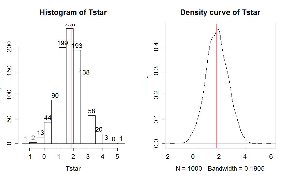
The permutation distribution in the same situation (Figure 1-12) had a similar shape but was centered at 0. Permutations create distributions based on assuming the null hypothesis is true, which is useful for hypothesis testing. Bootstrapping creates distributions centered at the observed result, sort of like distributions under the alternative; bootstrap distributions are useful for generating intervals for the true parameter values.
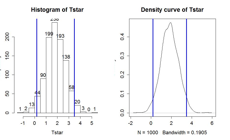
To create a 95% bootstrap confidence interval for the difference in the true mean sentences (μUnattr - μAve), we select the middle 95% of results from the bootstrap distribution. Specifically, we find the 2.5th percentile and the 97.5th percentile (values that put 2.5 and 97.5% of the results to the left), which leaves 95% in the middle. To find percentiles in a distribution, we will use functions that are q[Name of distribution] and from the bootstrap results we will use the qdata function on the Tstar results.
> qdata(.025,Tstar)
p quantile
0.0250000 0.1914578
> qdata(.975,Tstar)
p quantile
0.975000 3.484155
These results tell us that the 2.5th percentile of the bootstrap distribution is at 0.19 years and the 97.5th percentile is at 3.48 years. We can combine these results to provide a 95% confidence for μUnattr - μAve that is between 0.19 and 3.48. We can interpret this as with any confidence interval, that we are 95% confident that the difference in the true means (Unattractive minus Average) is between 0.19 and 3.48 years. We can also obtain both percentiles in one line of code using:
> quantiles<-qdata(c(.025,.975),Tstar)
> quantiles
quantile p
2.5% 0.1914578 0.025
97.5% 3.4841547 0.975
Figure 1-18 displays those same percentiles on the same bootstrap distribution.
> hist(Tstar,labels=T)
> abline(v=quantiles$quantile,col="blue",lwd=3)
> plot(density(Tstar),main="Density curve of Tstar")
> abline(v=quantiles$quantile,col="blue",lwd=3)
Although confidence intervals can exist without referencing hypotheses, we can revisit our previous hypotheses and see what this confidence interval tells us about the test of H0: μUnattr = μAve. This null hypothesis is equivalent to testing H0: μUnattr - μAve=0, that the difference in the true means is equal to 0 years. And the difference in the means was the scale for our confidence interval, which did not contain 0 years. We will call 0 an interesting reference value for the confidence interval, because here it is the value where the true means are equal other (have a difference of 0 years). In general, if our confidence interval does not contain 0, then it is saying that 0 is not one of our likely values for the difference in the true means. This implies that we should reject a claim that they are equal. This provides the same inferences for the hypotheses that we considered previously using both a parametric and permutation approach. The general summary is that we can use confidence intervals to test hypotheses by assessing whether the reference value under the null hypothesis is in the confidence interval (FTR H0) or outside the confidence interval (Reject H0).
As in the previous situation, we also want to consider the parametric approach for comparison purposes and to have that method available for the rest of the semester. The parametric confidence interval is called the equal variance, two-sample t-based confidence interval and assumes that the populations being sampled from are normally distributed and leads to using a t-distribution to form the interval. The output from the t.test function provides the parametric 95% confidence interval calculated for you:
> t.test(Years ~ Attr, data=MockJury2,var.equal=T)
Two Sample t-test
data: Years by Attr
t = -2.1702, df = 73, p-value = 0.03324
alternative hypothesis: true difference in means is not equal to 0
9
5 percent confidence interval:
-3.5242237 -0.1500295
sample estimates:
| mean in group Average | mean in group Unattractive |
| 3.973684 | 5.810811 |
The t.test function again switched the order of the groups and provides slightly different end-points than our bootstrap confidence interval (both made at the 95% confidence level), which was slightly narrower. Both intervals have the same interpretation, only the methods for calculating the intervals and the assumptions differ. Specifically, the bootstrap interval can tolerate different distribution shapes other than normal and still provide intervals that work well. The other assumptions are all the same as for the hypothesis test, where we continue to assume that we have independent observations with equal variances for the two groups.
The formula that t.test is using to calculate the parametric equal-variance two-sample t-based confidence interval is:

In this situation, the df is again n1+n2−2 and  The t*df is a multiplier that comes from finding the percentile from the t-distribution that puts C% in the middle of the distribution with C being the confidence level. It is important to note that this t* has nothing to do with the previous test statistic t. It is confusing and many of you will, at some point, happily take the result from a test statistic calculation and use it for a multiplier in a t-based confidence interval. Figure 1-19 shows the t-distribution with 73 degrees of freedom and the cut-offs that put 95% of the area in the middle.

For 95% confidence intervals, the multiplier is going to be close to 2 - anything else is a sign of a mistake. We can use R to get the multipliers for us using the qt function in a similar fashion to how we used qdata in the bootstrap results, except that this new value must be used in the previous formula. This function produces values for requested percentiles. So if we want to put 95% in the middle, we place 2.5% in each tail of the distribution and need to request the 97.5th percentile. Because the t-distribution is always symmetric around 0, we merely need to look up the value for the 97.5th percentile. The t* multiplier to form the confidence interval is 1.993 for a 95% confidence interval when the df=73 based on the results from qt:
> qt(.975,df=73)
[1] 1.992997
Note that the 2.5th percentile is just the negative of this value due to symmetry and the real source of the minus in the plus/minus in the formula for the confidence interval.
> qt(.025,df=73)
[1] -1.992997
We can also re-write the general confidence interval formula more simply as

where  In some situations, researchers will report the standard error (SE) or margin of error (ME) as a method of quantifying the uncertainty in a statistic. The SE is an estimate of the standard deviation of the statistic (here x1−x2) and the ME is an estimate of the precision of a statistic that can be used to directly form a confidence interval. The ME depends on the choice of confidence level although 95% is almost always selected.
To finish this example, we can use R to help us do calculations much like a calculator except with much more power "under the hood". You have to make sure you are careful with using ( ) to group items and remember that the asterisk (*) is used for multiplication. To do this, we need the pertinent information which is available from the bolded parts of the favstats output repeated below.
> favstats(Years~Attr,data=MockJury2)
| min | Q1 | median | Q3 | max | mean | sd | n | missing | |
| Average | 1 | 2 | 3 | 5 | 12 | 3.973684 | 2.823519 | 38 | 0 |
| Unattractive | 1 | 2 | 5 | 10 | 15 | 5.810811 | 4.364235 | 37 | 0 |
We can start with typing the following command to calculate sp:
> sp <- sqrt(((38-1)*(2.8235^2)+(37-1)*(4.364^2))/(38+37-2))
> sp
[1] 3.665036
So then we can calculate the confidence interval that t.test provided using:
> 3.974-5.811+c(-1,1)*qt(.975,df=73)*sp*sqrt(1/38+1/37)
[1] -3.5240302 -0.1499698
The previous code uses c(-1,1) times the margin of error to subtract and add the ME to the difference in the sample means (3.974-5.811) to generate the lower and then upper bounds of the confidence interval. If desired, we can also use just the last portion of the previous calculation to find the margin of error, which is 1.69 here.
> qt(.975,df=73)*sp*sqrt(1/38+1/37)
[1] 1.68703