1.6 - Second example of permutation tests
by
In every chapter, we will follow the first example used to explain the methods with a "worked" example where we focus on the results provided. In a previous semester, some of the STAT 217 students (n=79) provided information on their gender, Age, and current GPA. We might be interested in whether Males and Females had different average GPAs. First, we can take a look at the difference in the responses by groups as displayed in Figure 1-15.
> s217=read.csv( http://dl.dropboxusercontent.com/u/77307195/s217.csv)
> require(mosaic)
> par(mfrow=c(1,2))
> boxplot(GPA~Sex,data=s217)
> require(beanplot)
> beanplot(GPA~Sex,data=s217, log="",col="lightblue",method="jitter")
>
> mean(GPA~Sex,data=s217)
| F | M |
| 3.338378 | 3.088571 |
> favstats(GPA~Sex,data=s217)
| .group | min | Q1 | median | Q3 | max | mean | sd | n | missing | |
| 1 | F | 2.50 | 3.1 | 3.400 | 3.70 | 4 | 3.338378 | 0.4074549 | 37 | 0 |
| 2 | M | 1.96 | 2.8 | 3.175 | 3.46 | 4 | 3.088571 | 0.4151789 | 42 | 0 |
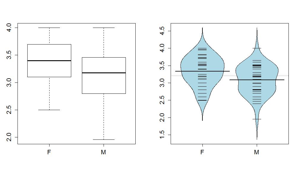
In these data, the distributions of the GPAs look to be left skewed but maybe not as dramatically as the responses were right-skewed in the previous example. The Female GPAs look to be slightly higher than for Males (0.25 GPA difference in the means) but is that a "real" difference? We need our inference tools to more fully assess these differences.
> compareMean(GPA~Sex,data=s217)
[1] -0.2498069
First, we can try the parametric approach:
> t.test(GPA~Sex,data=s217,var.equal=T)
Two Sample t-test
data: GPA by Sex
t = 2.6919, df = 77, p-value = 0.008713
alternative hypothesis: true difference in means is not equal to 0
95 percent confidence interval:
0.06501838 0.43459552
sample estimates:
| mean in group F | mean in group M |
| 3.338378 | 3.088571 |
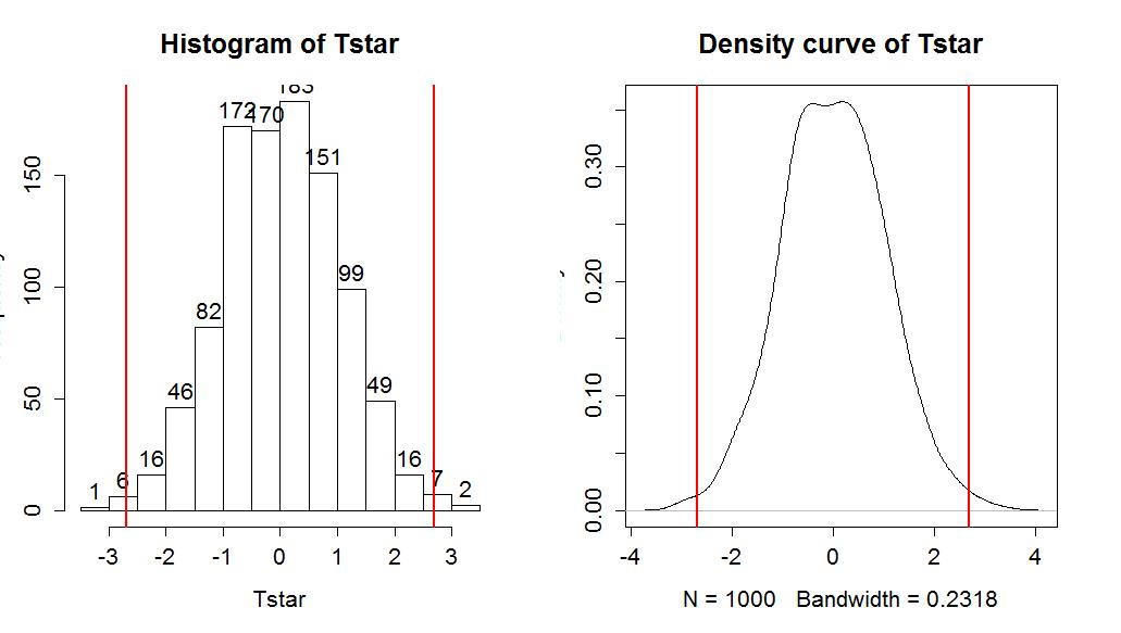
So the test statistic was observed to be t=2.69 and it hopefully follows a t(77) distribution under the null hypothesis. This provides a p-value of 0.008713 that we can trust if all of the conditions are met. We can compare these results to the permutation approach, which relaxes that normality assumption, with the required code and results following. In the permutation test, T=2.692 and the p-value is 0.011 which is a little larger than the result provided by the parametric approach. The agreement of the two approaches provides some re-assurance about the use of either approach.
> Tobs <- t.test(GPA~Sex,data=s217,var.equal=T)$statistic
> Tobs
t
2.691883
> Tstar<-matrix(NA,nrow=B)
> for (b in (1:B)){
+ Tstar[b]<-t.test(GPA~shuffle(Sex),data=s217,var.equal=T)$statistic
+ }
> hist(Tstar,labels=T)
> abline(v=c(-1,1)*Tobs,lwd=2,col="red")
> plot(density(Tstar),main="Density curve of Tstar")
> abline(v=c(-1,1)*Tobs,lwd=2,col="red")
> pdata(abs(Tobs),abs(Tstar),lower.tail=F)
t
0.011
Here is a full write-up of the results using all 6+ hypothesis testing steps, using the permutation results:
Isolate the claim to be proved and method to use (define a test statistic T)We want to test for a difference in the means between males and females and will use the equal-variance two-sample t-test statistic to compare them, making a decision at the 5% significance level.
1) Write the null and alternative hypotheses
- •H0: μMale = μFemale
- ◦where μMale is the true mean GPA for males and μFemale is true mean GPA for females
- •HA: μMale ≠ μFemale
2) Check conditions for the procedure being used
- •Independent observations condition: It appears that this assumption is met because there is no reason to assume any clustering or grouping of responses that might create dependence in the observations. The only possible consideration is that the observations were taken from different sections and there could be some differences between the sections. However, for overall GPA this not likely to be a big issue. The only way this could create a violation here is if certain sections tended to attract students with different GPA levels (such as the 9 am section had the best/worst GPA students...).
- •Equal variance condition: There is a small difference in the range of the observations in the two groups but the standard deviations are very similar so there is no evidence that this condition is violated.
- •Similar distribution condition: Based on the side-by-side boxplots and beanplots, it appears that both groups have slightly left-skewed distributions which could be problematic for the parametric approach but the permutation approach condition is not violated since the distributions look to have fairly similar shapes.
3) Find the value of the appropriate test statistic
- •T=2.69 from the previous R output
4) Find the p-value
- •p-value=0.012 from the permutation distribution results.
- •This means that there is about a 1.2% chance we would observe a difference in mean GPA (female-male or male-female) of 0.25 points or more if there in fact no difference in true mean GPA between females and males in STAT 217 in a particular semester.
5) Decision
- •Since the p-value is "small" (a priori 5% significance level selected), we can reject the null hypothesis.
6) Conclusion and scope of inference, specific to the problem
- •There is evidence against the null hypothesis of no difference in the true mean GPA between males and females for the STAT 217 students in this semester and so we conclude that there is evidence of a difference in the mean GPAs between males and females.
- •Because this was not a randomized experiment, we can't say that the difference in sex causes the difference in mean GPA and because it was not a random sample from a larger population, our inferences only pertain the STAT 217 students that responded to the survey in that semester.