1.5 - Connecting randomization (nonparametric) and parametric tests
by
In developing statistical inference techniques, we need to define the test statistic, T, that measures the quantity of interest. To compare the means of two groups, a statistic is needed that measures their differences. In general, for comparing two groups, the choices are simple - a difference in the means often works well and is a natural choice. There are other options such as tracking the ratio of means or possibly the difference in medians. Instead of just using the difference in the means, we could "standardize" the difference in the means by dividing by an appropriate quantity. It ends up that there are many possibilities for testing using the randomization (nonparametric) techniques introduced previously. Parametric statistical methods focus on means because the statistical theory surrounding means is quite a bit easier (not easy, just easier) than other options. Randomization techniques allow inference for other quantities but our focus here will be on using randomization for inferences on means to see the similarities with the more traditional parametric procedures.
In two-sample mean situations, instead of working with the difference in the means, we often calculate a test statistic that is called the equal variance two-independent samples t-statistic. The test statistic is

where s12 and s22 are the sample variances for the two groups, n1 and n2 are the sample sizes for the two groups, and the pooled sample standard devation,
The t-statistic keeps the important comparison between the means in the numerator that we used before and standardizes (re-scales) that difference so that t will follow a t-distribution (a parametric "named" distribution) if certain assumptions are met. But first we should see if standardizing the difference in the means had an impact on our permutation test results. Instead of using the compareMean function, we will use the t.test function (see its full use below) and have it calculate the formula for t for us. The R code "$statistic" is basically a way of extracting just the number we want to use for T from a larger set of output the t.test function wants to provide you. We will see below that t.test switches the order of the difference (now it is Average - Unattractive) - always carefully check for the direction of the difference in the results. Since we are doing a two-sided test, the code resembles the permutation test code in Section 1.3 with the new t-statistic replacing the difference in the sample means.
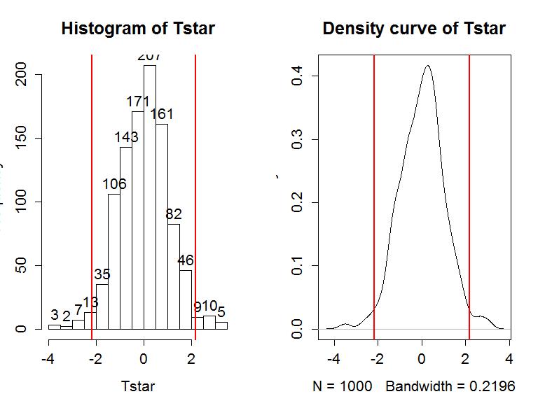
The permutation distribution in Figure 1-12 looks similar to the previous results with slightly different x-axis scaling. The observed t-statistic was -2.17 and the proportion of permuted results that were more extreme than the observed result was 0.034. This difference is due to a different set of random permutations being selected. If you run permutation code, you will often get slightly different results each time you run it. If you are uncomfortable with the variation in the results, you can run more than B=1,000 permutations (say 10,000) and the variability will be reduced further. Usually this uncertainty will not cause any substantive problems - but do not be surprised if your results vary from a colleagues if you are both analyzing the same data set.
> Tobs <- t.test(Years ~ Attr, data=MockJury2,var.equal=T)$statistic
> Tobs
t
-2.17023
> Tstar<-matrix(NA,nrow=B)
> for (b in (1:B)){
+ Tstar[b]<-t.test(Years ~ shuffle(Attr), data=MockJury2,var.equal=T)$statistic
+ }
> hist(Tstar,labels=T)
> abline(v=c(-1,1)*Tobs,lwd=2,col="red")
> plot(density(Tstar),main="Density curve of Tstar")
> abline(v=c(-1,1)*Tobs,lwd=2,col="red")
>
> pdata(abs(Tobs),abs(Tstar),lower.tail=F)
t
0.034
The parametric version of these results is based on using what is called the two-independent sample t-test. There are actually two versions of this test, one that assumes that variances are equal in the groups and one that does not. There is a rule of thumb that if the ratio of the larger standard deviation over the smaller standard deviation is less than 2, the equal variance procedure is ok. It ends up that this assumption is less important if the sample sizes in the groups are approximately equal and more important if the groups contain different numbers of observations. In comparing the two potential test statistics, the procedure that assumes equal variances has a complicated denominator (see the formula above for t involving sp) but a simple formula for degrees of freedom (df) for the t-distribution (df=n1+n2−2) that approximates the distribution of the test statistic, t, under the null hypothesis. The procedure that assumes unequal variances has a simpler test statistic and a very complicated degrees of freedom formula. The equal variance procedure is most similar to the ANOVA methods we will consider later this semester so that will be our focus here. Fortunately, both of these methods are readily available in the t.test function in R if needed.
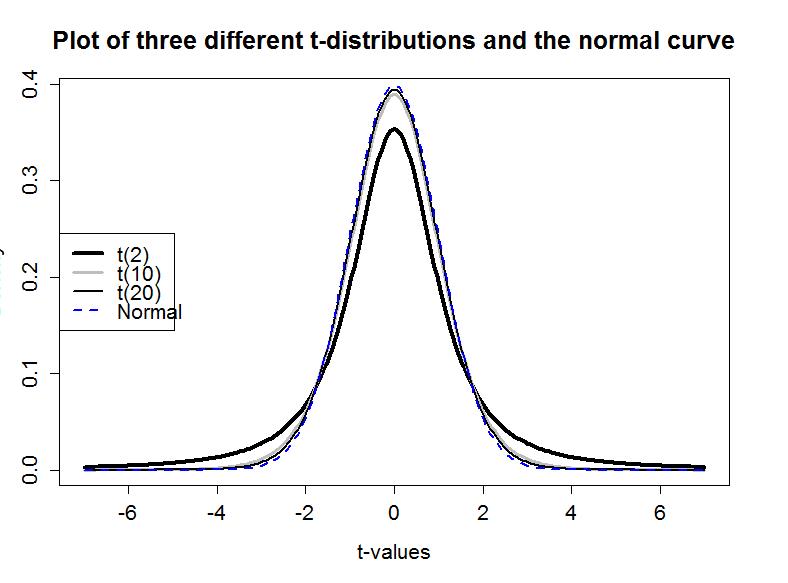
If the assumptions for the equal variance t-test are met and the null hypothesis is true, then the sampling distribution of the test statistic should follow a t-distribution with n1+n2−2 degrees of freedom. The t-distribution is a bell-shaped curve that is more spread out for smaller values of degrees of freedom as shown in Figure 1-13. The t-distribution looks more and more like a standard normal distribution (N(0,1)) as the degrees of freedom increase.
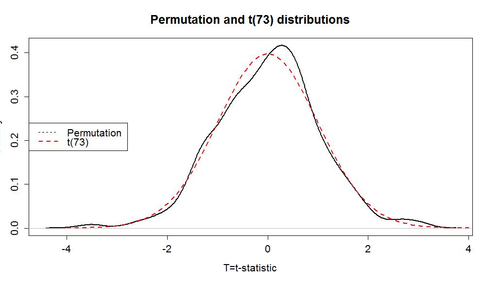
To get the p-value from the parametric t-test, we need to calculate the test statistic and df, then look up the areas in the tails of the t-distribution relative to the observed t-statistic. We'll learn how to use R to do this below, but for now we will allow the t.test function to take care of this for us. The t.test function uses our formula notation (Years ~ Attr) and then data=... as we saw before for making plots. To get the equal-variance test result, the var.equal=T option needs to be turned on. Then t.test provides us with lots of useful output. We highlighted the three results we've been discussing - the test statistic value (-2.17), df=73, and the p-value, from the t-distribution with 73 degrees of freedom, of 0.033.
> t.test(Years ~ Attr, data=MockJury2,var.equal=T)
Two Sample t-test data: Years by Attr t = -2.1702, df = 73, p-value = 0.03324 alternative hypothesis: true difference in means is not equal to 0 95 percent confidence interval: -3.5242237 -0.1500295 sample estimates: So the parametric t-test gives a p-value of 0.033 from a test statistic of -2.1702. The negative sign on the statistic occurred because the function took Average - Unattractive which is the opposite direction as compareMeans. The p-value is very similar to the two permutation results found before. The reason for this similarity is that the permutation distribution looks an awful lot like a t-distribution with 73 degrees of freedom. Figure 1-14 shows how similar the two distributions happened to be here. In your previous statistics course, you might have used an applet or a table to find p-values such as what was provided in the previous R output. When not directly provided by a function, we will use R to find p-values 18 from named distributions such as the t-distribution. In this case, the distribution is a t(73) or a t with 73 degrees of freedom. We will use the pt function to get p-values from the t-distribution in the same manner as we used pdata to find p-values from the permutation distribution. We need to provide the df=... and specify the tail of the distribution of interest using the lower.tail option. If we want the area to the left of -2.17: > pt(-2.1702,df=73,lower.tail=T) [1] 0.01662286 And we can double it to get the p-value that t.test provided earlier, because the t-distribution is symmetric: > 2*pt(-2.1702,df=73,lower.tail=T) [1] 0.03324571 More generally, we could always make the test statistic positive using the absolute value, find the area to the right of it, and then double that for a two-side test p-value: > 2*pt(abs(-2.1702),df=73,lower.tail=F) [1] 0.03324571 Permutation distributions do not need to match the named parametric distribution to work correctly, although this happened in the previous example. The parametric approach, the t-test, requires the certain conditions to be met for the sampling distribution of the statistic to follow the named distribution and provide accurate p-values. The conditions for the equal variance t-test are: 1) Independent observations: Each observation obtained is unrelated to all other observations. To assess this, consider whether there anything in the data collection might lead to clustered or related observations that are un-related to the differences in the groups. For example, was the same person measured more than once?19 2) Equal variances in the groups (because we used a procedure that assumes equal variances! - there is another procedure that allows you to relax this assumption if needed...). To assess this, compare the standard deviations and see if they look noticeably different, especially if the sample sizes differ between groups. 3) Normal distributions of the observations in each group. We'll learn more diagnostics later, but the boxplots and beanplots are a good place to start to help you look for skews or outliers, which were both present here. If you find skew and/or outliers, that would suggest a problem with this condition. For the permutation test, we relax the third condition: 3) Similar distributions between the groups: The permutation approach helps us with this assumption and allows valid inferences as long as the two groups have similar shapes and only possibly differ in their centers. In other words, the distributions need not look normal for the procedure to work well. In the mock jury study, we can assume that the independent observation condition is met because there is no information suggesting that the same subjects were measured more than once or that some other type of grouping in the responses was present (like the subjects were divided in groups and placed in the same room discussing their responses). The equal variance condition might be violated although we do get some lee-way in this assumption and are still able to get reasonable results. The standard deviations are 2.8 vs 4.4, so this difference is not "large" according to the rule of thumb. It is, however, close to being considered problematic. It would be difficult to reasonably assume that the the normality condition is met here (Figure 1-6), that is assumed in the derivation of the parametric procedure, with clear right skews in both groups and potential outliers. The shapes look similar for the two groups so there is less reason to be concerned with using the permutation approach as compared to the parametric approach. The permutation approach is resistant to impacts of violations of the normality assumption. It is not resistant to impact of violations of any of the other assumptions. In fact, it can be quite sensitive to unequal variances as it will detect differences in the variances of the groups instead of differences in the means. Its scope of inference is limited just like the parametric approach and can lead to similarly inaccurate conclusions in the presence of non-independent observations as for the parametric approach. For our purposes, we hope that seeing the similarity in the methods can help you understand both methods better. In this example, we discover that parametric and permutation approaches provide very similar inferences. 18 On exams, you will be asked to describe the area of interest, sketch a picture of the area of interest and/or note the distribution you would use. 19 In some studies, the same subject might be measured in both conditions and this violates the assumptions of this procedure.
mean in group Average mean in group Unattractive 3.973684 5.810811