1.2 - Models, hypotheses, and permutations for the 2 sample mean situation
by
There appears to be some evidence that the Unattractive group is getting higher average lengths of sentences from the mock jurors than the Average group, but we want to make sure that the difference is real - that there is evidence to reject the assumption that the means are the same "in the population". First, a null hypothesis11 which defines a null model12 needs to be determined in terms of parameters (the true values in the population). The research question should help you determine the form of the hypotheses for the assumed population. In the 2 independent sample mean problem, the interest is in testing a null hypothesis of H0: μ1=μ2 versus the alternative hypothesis of HA: μ1≠μ2, where μ1 is the parameter for the true mean of the first group and μ2 is the parameter for the true mean of the second group. The alternative hypothesis involves assuming a statistical model for the ith (i=1,...,nj) response from the jth group (j=1,2), γij, is modeled as γij = μj + εij, where we typically assume that εij ~ N(0,σ2). For the moment, focus on the models that assuming the means are the same (null) or different (alternative) imply:
| • | Null Model: γij = μ + εij | There is no difference in true means for the two groups. |
|---|---|---|
| • | Alternative Model: yij = μj + εij | There is a difference in true means for the two groups. |
Suppose we are considering the alternative model for the 4th observation (i=4) from the second group (j=2), then the model for this observation is γ42 = μ2 + ε42. And for, say, the 5th observation from the first group (j=1), the model is γ51 = μ1 + ε51. If we were working with the null model, the mean is always the same (μ) and the group specified does not change that aspect of the model.
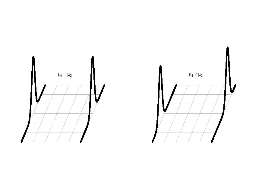
It can be helpful to think about the null and alternative models graphically. By assuming the null hypothesis is true (means are equal) and that the random errors around the mean follow a normal distribution, we assume that the truth is as displayed in the left panel of Figure 1-7 - two normal distributions with the same mean and variability. The alternative model allows the two groups to potentially have different means, such as those displayed in the right panel of Figure 1-7, but otherwise assumes that the responses have the same distribution. We assume that the observations (γij) would either have been generated as samples from the null or alternative model - imagine drawing observations at random from the pictured distributions. The hypothesis testing task in this situation involves first assuming that the null model is true and then assessing how unusual the actual result was relative to that assumption so that we can conclude that the alternative model is likely correct. The researchers obviously would have hoped to encounter some sort of noticeable difference in the sentences provided for the different pictures and been able to find enough evidence to reject the null model where the groups "looked the same".
In statistical inference, null hypotheses (and their implied models) are set up as "straw men" with every interest in rejecting them even though we assume they are true to be able to assess the evidence against them. Consider the original study design here, the pictures were randomly assigned to the subjects. If the null hypothesis were true, then we would have no difference in the population means of the groups. And this would apply if we had done a different random assignment of the pictures to the subjects. So let's try this: assume that the null hypothesis is true and randomly re-assign the treatments (pictures) to the observations that were obtained. In other words, keep the sentences (Years) the same and shuffle the group labels randomly. The technical term for this is doing a permutation (a random shuffling of the treatments relative to the responses). If the null is true and the means in the two groups are the same, then we should be able to re-shuffle the groups to the observed sentences (Years) and get results similar to those we actually observed. If the null is false and the means are really different in the two groups, then what we observed should differ from what we get under other random permutations. The differences between the two groups should be more noticeable in the observed data set than in (most) of the shuffled data sets. It helps to see this to understand what a permutation means in this context.
In the mosaic R package, the shuffle function allows us to easily perform a permutation13. Just one time, we can explore what a permutation of the treatment labels could look like.
> Perm1 <- with(MockJury2,data.frame(Years,Attr,PermutedAttr=shuffle(Attr)))
> Perm1
| Years | Attr | PermutedAttr | |
|---|---|---|---|
| 1 | 1 | Unattractive | Unattractive |
| 2 | 4 | Unattractive | Average |
| 3 | 3 | Unattractive | Average |
| 4 | 2 | Unattractive | Average |
| 5 | 8 | Unattractive | Unattractive |
| 6 | 8 | Unattractive | Unattractive |
| 7 | 1 | Unattractive | Unattractive |
| 8 | 1 | Unattractive | Unattractive |
| 9 | 5 | Unattractive | Unattractive |
| 10 | 7 | Unattractive | Unattractive |
| 11 | 1 | Unattractive | Average |
| 12 | 5 | Unattractive | Unattractive |
| 13 | 2 | Unattractive | Unattractive |
| 14 | 12 | Unattractive | Unattractive |
| 15 | 10 | Unattractive | Unattractive |
| 16 | 1 | Unattractive | Average |
| 17 | 6 | Unattractive | Average |
| 18 | 2 | Unattractive | Average |
| 19 | 5 | Unattractive | Average |
| 20 | 12 | Unattractive | Average |
| 21 | 6 | Unattractive | Average |
| 22 | 3 | Unattractive | Average |
| 23 | 8 | Unattractive | Unattractive |
| 24 | 4 | Unattractive | Unattractive |
| 25 | 10 | Unattractive | Average |
| 26 | 10 | Unattractive | Unattractive |
| 27 | 15 | Unattractive | Unattractive |
| 28 | 15 | Unattractive | Unattractive |
| 29 | 3 | Unattractive | Average | 30 | 3 | Unattractive | Unattractive |
| 31 | 3 | Unattractive | Average |
| 32 | 11 | Unattractive | Average |
| 33 | 12 | Unattractive | Average |
| 34 | 2 | Unattractive | Unattractive |
| 35 | 1 | Unattractive | Average |
| 36 | 1 | Unattractive | Average |
| 37 | 12 | Unattractive | Unattractive |
| 38 | 5 | Average | Average |
| 39 | 5 | Average | Average |
| 40 | 4 | Average | Unattractive |
| 41 | 3 | Average | Unattractive |
| 42 | 6 | Average | Average |
| 43 | 4 | Average | Average |
| 44 | 9 | Average | Unattractive |
| 45 | 8 | Average | Average |
| 46 | 3 | Average | Unattractive |
| 47 | 2 | Average | Average |
| 48 | 10 | Average | Average |
| 49 | 1 | Average | Unattractive |
| 50 | 1 | Average | Unattractive |
| 51 | 3 | Average | Unattractive |
| 52 | 1 | Average | Unattractive |
| 53 | 3 | Average | Unattractive |
| 54 | 5 | Average | Unattractive |
| 55 | 8 | Average | Unattractive |
| 56 | 3 | Average | Average |
| 57 | 1 | Average | Average |
| 58 | 1 | Average | Average |
| 59 | 1 | Average | Average |
| 60 | 2 | Average | Average |
| 61 | 2 | Average | Unattractive |
| 62 | 1 | Average | Average |
| 63 | 1 | Average | Unattractive |
| 64 | 2 | Average | Average |
| 65 | 3 | Average | Unattractive |
| 66 | 4 | Average | Unattractive |
| 67 | 5 | Average | Average |
| 68 | 3 | Average | Unattractive |
| 69 | 3 | Average | Unattractive |
| 70 | 3 | Average | Average |
| 71 | 2 | Average | Average |
| 72 | 7 | Average | Unattractive |
| 73 | 6 | Average | Average |
| 74 | 12 | Average | Average |
| 75 | 8 | Average | Average |
If you count up the number of subjects in each group by counting the number of times each label (Average, Unattractive) occurs, it is the same in both the Attr and PermutedAttr columns. Permutations involve randomly re-ordering the values of a variable - here the Attr group labels. This result can also be generated using what is called sampling without replacement: sequentially select n labels from the original variable, removing each used label and making sure that each original Attr label is selected once and only once. The new, randomly selected order of selected labels provides the permuted labels. Stepping through the process helps us understand how it works: after the initial random sample of one label, there would n-1 choices possible; on the nth selection, there would only be one label remaining to select. This makes sure that all original labels are re-used but that the order is random. Sampling without replacement is like picking names out of a hat, one-at-a-time, and not putting the names back in after they are selected. Sampling with replacement involves sampling from the specified list with each observation having an equal chance of selection for each sampled observation - in other words, observations can be selected more than once. This is like picking n names out of a hat that contains n names, except that every time a name is selected, it goes back into the hat - we'll use this technique later in the Chapter to do what is called bootstrapping. Both sampling mechanisms can be used to generate inferences but each has particular situations where they are most useful.
The comparison of the beanplots for the real data set and permuted version of the labels is what is really interesting (Figure 1-8). The original difference in the sample means of the two groups was 1.84 years (Unattractive minus Average). The sample means are the statistics that estimate the parameters for the true means of the two groups. In the permuted data set, the difference in the means is 0.66 years.
> mean(Years ~ PermutedAttr, data=Perm1)
| Average | Unattractive |
|---|---|
| 4.552632 | 5.216216 |
> compareMean(Years ~ PermutedAttr, data=Perm1)
[1] 0.6635846
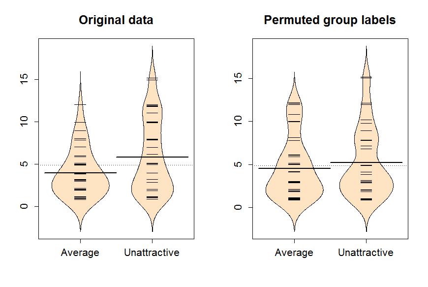
These results suggest that the observed difference was larger than what we got when we did a single permutation. The important aspect of this is that the permutation is valid if the null hypothesis is true - this is a technique to generate results that we might have gotten if the null hypothesis were true. We just need to repeat the permutation process many times and track how unusual our observed result is relative to this distribution of responses. If the observed differences are unusual relative to the results under permutations, then there is evidence against the null hypothesis, the null hypothesis should be rejected (Reject H0) and a conclusion should be made, in the direction of the alternative hypothesis, that there is evidence that the true means differ. If the observed differences are similar to (or at least not unusual relative to) what we get under random shuffling under the null model, we would have a tough time concluding that there is any real difference between the groups based on our observed data set.
11The hypothesis of no difference that is typically generated in the hopes of being rejected in favor of the alternative hypothesis which contains the sort of difference that is of interest in the application.
12The null model is the statistical model that is implied by the chosen null hypothesis. Here, a null hypothesis of no difference will translate to having a model with the same mean for both groups.
13We'll see the shuffle function in a more common usage below; while the code to generate Perm1 is provided, it isn't something to worry about right now: Perm1<-with(MockJury2,data.frame(Years,Attr,PermutedAttr=shuffle(Attr)))