1.3 - Permutation testing for the 2 sample mean situation
by
In any testing situation, you must define some function of the observations that gives us a single number that addresses our question of interest. This quantity is called a test statistic. These often take on complicated forms and have names like t or z statistics that relate to their parametric (named) distributions so we know where to look up p-values. In randomization settings, they can have simpler forms because we use the data set to find the distribution of the statistic. We will label our test statistic T (for Test statistic) unless the test statistic has a commonly used name. Since we are interested in comparing the means of the two groups, we can define T=xUnattractive−xAverage, which coincidentally is what the compareMean function provided us previously. We label our observed test statistic (the one from the original data set) as Tobs=xUnattractive−xAverage which happened to be 1.84 years here. We will compare this result to the results for the test statistic that we obtain from permuting the group labels. To denote permuted results, we will add a * to the labels: T*=xUnattractive*−xAverage*. We then compare the Tobs=xUnattractive−xAverage= 1.84 to the distribution of results that are possible for the permuted results (T*) which corresponds to assuming the null hypothesis is true.
To do permutations, we are going to learn how to write a for loop in R to be able to repeatedly generate the permuted data sets and record T*. Loops are a basic programming task that make randomization methods possible as well as potentially simplifying any repetitive computing task. To write a "for loop", we need to choose how many times we want to do the loop (call that B) and decide on a counter to keep track of where we are at in the loops (call that b, which goes from 1 to B). The simplest loop would just involve printing out the index, print(b). This is our first use of curly braces, { and }, that are used to group the code we want to repeatedly run as we proceed through the loop. The code in the script window is:
for (b in (1:B)){
print(b)
}
And when you highlight and run the code, it will look about the same with "+" printed after the first line to indicate that all the code is connected, looking like this:
> for (b in (1:B)){
+ print(b)
+ }
When you run these three lines of code, the console will show you the following output:
| [1] | 1 |
| [1] | 2 |
| [1] | 3 |
| [1] | 4 |
| [1] | 5 |
This is basically the result of running the print function on b as it has values from 1 to 5.
Instead of printing the counter, we want to use the loop to repeatedly compute our test statistic when permuting observations. The shuffle function will perform permutations of the group labels relative to responses and the compareMean function will calculate the difference in two group means. For a single permutation, the combination of shuffling Attr and finding the difference in the means, storing it in a variable called Ts is:
> Ts<-compareMean(Years ~ shuffle(Attr), data=MockJury2)
> Ts
[1] 0.3968706
And putting this inside the print function allows us to find the test statistic under 5 different permutations easily:
> for (b in (1:B)){
+ Ts<-compareMean(Years ~ shuffle(Attr), data=MockJury2)
+ print(Ts)
+ }
| [1] | 0.9302987 |
| [1] | 0.6635846 |
| [1] | 0.7702703 |
| [1] | -1.203414 |
| [1] | -0.7766714 |
Finally, we would like to store the values of the test statistic instead of just printing them out on each pass through the loop. To do this, we need to create a variable to store the results, let's call it Tstar. We know that we need to store B results so will create a vector of length B, containing B elements, full of missing values (NA) using the matrix function:
> Tstar<-matrix(NA,nrow=B)
> Tstar
| [,1] | |
| [1,] | NA |
| [2,] | NA |
| [3,] | NA |
| [4,] | NA |
| [5,] | NA |
Now we can run our loop B times and store the results in Tstar:
> for (b in (1:B)){
+ Tstar[b]<-compareMean(Years ~ shuffle(Attr), data=MockJury2)
+ }
> Tstar
| [,1] | |
| [1,] | 1.1436700 |
| [2,] | -0.7233286 |
| [3,] | 1.3036984 |
| [4,] | -1.1500711 |
| [5,] | -1.0433855 |
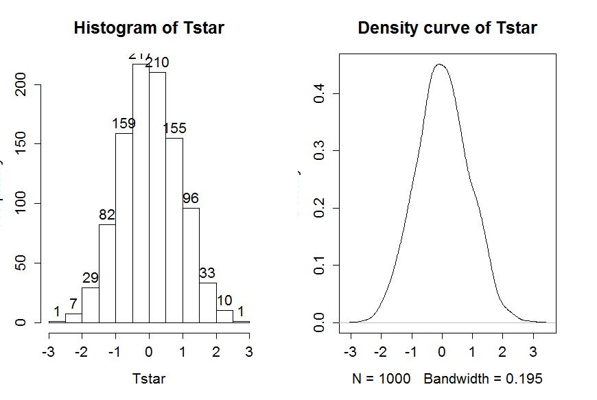
The Tstar vector when we set B to be large, say B=1,000, generate the permutation distribution for the selected test statistic under14the null hypothesis - what is called the null distribution of the statistic and also its sampling distribution. We want to visualize this distribution and use it to assess how unusual our Tobs result of 1.84 years was relative to all the possibilities under permutations (under the null hypothesis). So we repeat the loop, now with B=1000 and generate a histogram, density curve and summary statistics of the results:
> B<-1000
> Tstar<-matrix(NA,nrow=B)
> for (b in (1:B)){
+ Tstar[b]<-compareMean(Years ~ shuffle(Attr), data=MockJury2)
+ }
> hist(Tstar,labels=T)
> plot(density(Tstar),main="Density curve of Tstar")
> favstats(Tstar)
| min | Q1 | median | Q3 | max | mean | sd | n | missing |
| -2.536984 | -0.5633001 | 0.02347084 | 0.6102418 | 2.903983 | 0.01829659 | 0.8625767 | 1000 | 0 |
Figure 1-9 contains visualizations of the results for the distribution of T* and the favstats summary provides the related numerical summaries. Our observed Tobs of 1.837 seems fairly unusual relative to these results with only 11 T* values over 2 based on the histogram. We need to make more specific assessments of the permuted results versus our observed result to be able to clearly decide whether our observed result is really unusual.
We can enhance the previous graphs by adding the value of the test statistic from the real data set, as shown in Figure 1-10, using the abline function.
> hist(Tstar,labels=T)
> abline(v=Tobs,lwd=2,col="red")
> plot(density(Tstar),main="Density curve of Tstar")
> abline(v=Tobs,lwd=2,col="red")
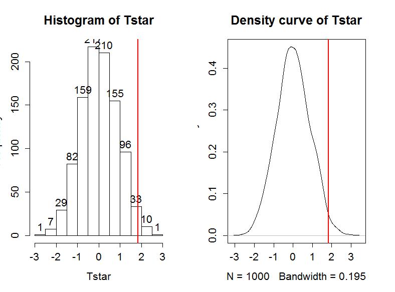
Second, we can calculate the exact number of permuted results that were larger than what we observed. To calculate the proportion of the 1,000 values that were larger than what we observed, we will use the pdata function. To use this function, we need to provide the cut-off point (Tobs), the distribution of values to compare to the cut-off (Tstar), and whether we want the lower or upper tail of the distribution (lower.tail=F option provides the proportion of values above).
> pdata(Tobs,Tstar,lower.tail=F)
[1] 0.016
The proportion of 0.016 tells us that 16 of the 1,000 permuted results (1.6%) were larger than what we observed. This type of work is how we can generate p-values using permutation distributions. P-values are the probability of getting a result as extreme or more extreme than what we observed, given that the null is true. Finding only 16 permutations of 1,000 that were larger than our observed result suggests that it is hard to find a result like what we observed if there really were no difference, although it is not impossible.
When testing hypotheses for two groups, there are two types of alternative hypotheses, one-sided or two-sided. One-sided tests involve only considering differences in one-direction (like μ1>μ2) and are performed when researchers can decide a priori15 which group should have a larger mean. We did not know enough about the potential impacts of the pictures to know which group should be larger than the other and without much knowledge we could have gotten the direction wrong relative to the observed results and we can't look at the responses to decide on the hypotheses. It is often safer and more conservative16 to start with a two-sided alternative (HA: μ1≠μ2). To do a 2-sided test, find the area larger than what we observed as above. We also need to add the area in the other tail (here the left tail) similar to what we observed in the right tail. Here we need to also find how many of the permuted results were smaller than -1.84 years, using pdata with -Tobs as the cut-off and lower.tail=T:
> pdata(-Tobs,Tstar,lower.tail=T)
[1] 0.015
So the p-value to test our null hypothesis of no difference in the true means between the groups is 0.016+0.015, providing a p-value of 0.031. Figure 1-11 shows both cut-offs on the histogram and density curve.
> hist(Tstar,labels=T)
> abline(v=c(-1,1)*Tobs,lwd=2,col="red")
> plot(density(Tstar),main="Density curve of Tstar")
> abline(v=c(-1,1)*Tobs,lwd=2,col="red")
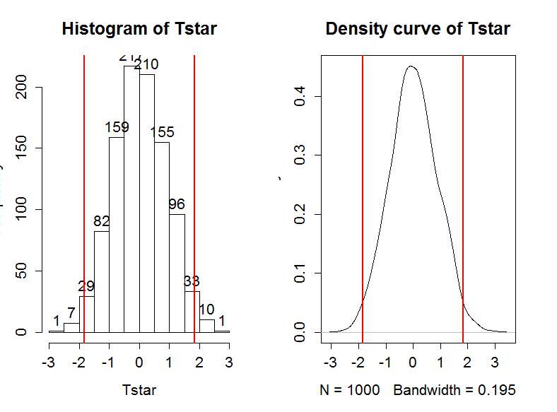
In general, the one-sided test p-value is the proportion of the permuted results that are more extreme than observed in the direction of the alternative hypothesis (lower or upper tail, which also depends on the direction of the difference taken). For the 2-sided test, the p-value is the proportion of the permuted results that are less than the negative version of the observed statistic and greater than the positive version of the observed statistic. Using absolute values, we can simplify this: the two-sided p-value is the proportion of the |permuted statistics| that are larger than |observed statistic|. This will always work and finds areas in both tails regardless of whether the observed statistic is positive or negative. In R, the abs function provides the absolute value and we can again use pdata to find our p-value:
> pdata(abs(Tobs),abs(Tstar),lower.tail=F)
[1] 0.031
We will discuss the choice of significance level below, but for the moment, assume a significance level (α) of 0.05. Since the p-value is smaller than α, this suggests that we can reject the null hypothesis and conclude that there is evidence of some difference in the true mean sentences given between the two types of pictures.
Before we move on, let's note some interesting features of the permutation distribution of the difference in the sample means shown in Figure 1-11.
Earlier, we decided that the p-value was small enough to reject the null hypothesis since it was smaller than our chosen level of significance. In this course, you will often be allowed to use your own judgement about an appropriate significance level in a particular situation (in other words, if we forget to tell you an α-level, you can still make a decision using a reasonably selected significance level). Remembering that the p-value is the probability you would observe a result like you did (or more extreme), assuming the null hypothesis is true, this tells you that the smaller the p-value is, the more evidence you have against the null. The next section provides a more formal review of the hypothesis testing infrastructure, terminology, and some of things that can happen when testing hypotheses.
14We often say "under" in statistics and we mean "given that the following is true".
15This is a fancy way of saying "in advance", here in advance of seeing the observations.
16Statistically, a conservative method is one that provides less chance of rejecting the null hypothesis in comparison to some other method or some pre-defined standard.
17We'll leave the discussion of the CLT to your previous stat coursework or an internet search.