1.1 - Beanplots
by
The other graphical display for comparing multiple groups we will use is a newer display called a beanplot (Kampstra, 2008). It provides a side-by-side display that contains the density curve, the original observations that generated the density curve in a rug-plot, and the mean of each group. For each group the density curves are mirrored to aid in visual assessment of the shape of the distribution. This mirroring will often create a shape that resembles a violin with skewed distributions. Long, bold horizontal lines are placed at the mean for each group. All together this plot shows us information on the center (mean), spread, and shape of the distributions of the responses. Our inferences typically focus on the means of the groups and this plot allows us to compare those across the groups while gaining information on whether the mean is reasonable summary of the center of the distribution.
To use the beanplot function we need to install and load the beanplot package. The function works like the boxplot used previously except that options for log, col, and method need to be specified. Use these options for any beanplots you make: log="",col="bisque", method="jitter".
> require(beanplot)
> beanplot(Years~Attr,data=MockJury,log="",col="bisque",method="jitter")
Figure 1-5 reinforces the strong right skews that were also detected in the boxplots previously. The three large sentences of 15 years can now be clearly viewed, one in the Beautiful group and two in the Unattractive group. The Unattractive group seems to have more high observations than the other groups even though the Beautiful group had the largest number of observations around 10 years. The mean sentence was highest for the Unattractive group and the differences differences in the means between Beautiful and Average was small.
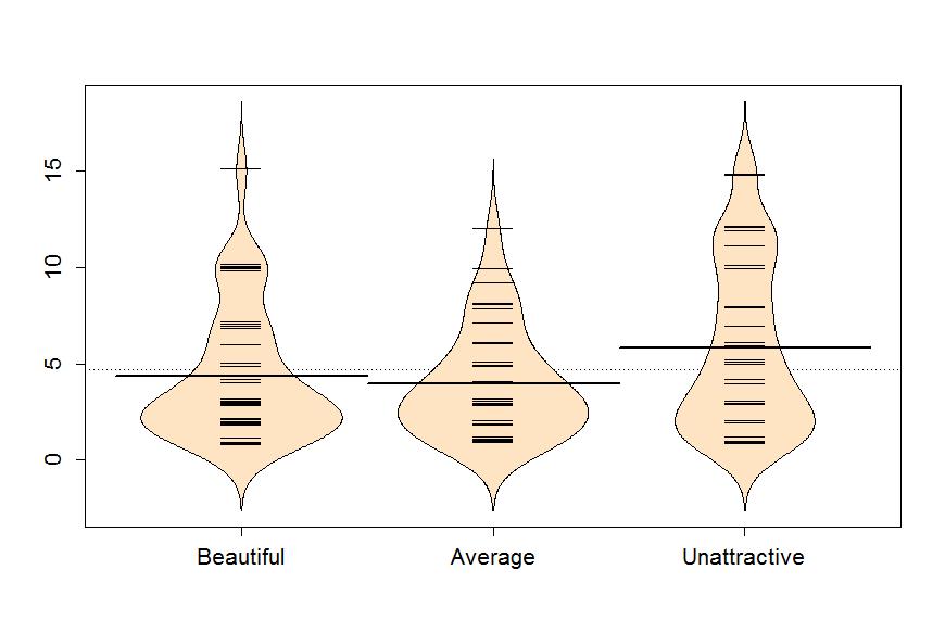
In this example, it appears that the mean for Unattractive is larger than the other two groups. But is this difference real? We will never know the answer to that question, but we can assess how likely we are to have seen a result as extreme or more extreme than our result, assuming that there is no difference in the means of the groups. And if the observed result is (extremely) unlikely to occur, then we can reject the hypothesis that the groups have the same mean and conclude that there is evidence of a real difference. We can get means and standard deviations by groups easily using the same formula notation with the mean and sd functions if the mosaic package is loaded.
> mean(Years~Attr,data=MockJuryR)
| Beautiful | Average | Unattractive |
| 4.333333 | 3.973684 | 5.810811 |
> sd(Years~Attr,data=MockJuryR)
| Beautiful | Average | Unattractive |
| 3.405362 | 2.823519 | 4.364235 |
We can also use the favstats function to get those summaries and others.
> favstats(Years~Attr,data=MockJuryR)
| min | Q1 | median | Q3 | max | mean | sd | n | missing | |
| Beautiful | 1 | 2 | 3 | 6.5 | 15 | 4.333333 | 3.405362 | 39 | 0 |
| Average | 1 | 2 | 3 | 5.0 | 12 | 3.973684 | 2.823519 | 38 | 0 |
| Unattractive | 1 | 2 | 5 | 10 | 15 | 5.810811 | 4.364235 | 37 | 0 |
We have an estimate of a difference of almost 2 years in the mean sentence between Average and Unattractive groups. Because there are three groups being compared in this study, we will have to wait to Chapter 2 and the One-Way ANOVA test to fully assess evidence related to some difference in the three groups. For now, we are going to focus on comparing the mean Years between Average and Unattractive groups - which is a 2 independent sample mean situation and something you have seen before. We will use this simple scenario to review some basic statistical concepts and connect two frameworks for conducting statistical inference, randomization and parametric techniques. Parametric statistical methods involve making assumptions about the distribution of the responses and obtaining confidence intervals and/or p-values using a named distribution (like the z or t-distributions). Typically these results are generated using formulas and looking up areas under curves using a table or a computer. Randomization-based statistical methods use a computer to shuffle, sample, or simulate observations in ways that allow you to obtain p-values and confidence intervals without resorting to using tables and named distributions. Randomization methods are what are called nonparametric methods that often make fewer assumptions (they are not free of assumptions!) and so can handle a larger set of problems more easily than parametric methods. When the assumptions involved in the parametric procedures are met, the randomization methods often provide very similar results to those provided by the parametric techniques. To be a more sophisticated statistical consumer, it is useful to have some knowledge of both of these approaches to statistical inference and the fact that they can provide similar results might deepen your understanding of both approaches.
Because comparing two groups is easier than comparing more than two groups, we will start with comparing the Average and Unattractive groups. We could remove the Beautiful group observations in a spreadsheet program and read that new data set back into R, but it is easier to use R to do data management once the data set is loaded. To remove the observations that came from the Beautiful group, we are going to generate a new variable that we will call NotBeautiful that is true when observations came from another group (Average or Unattractive) and false for observations from the Beautiful group. To do this, we will apply the not equal logical function (!=) to the variable Attr, inquiring whether it was different from the "Beautiful" level.
> NotBeautiful <- MockJury$Attr!="Beautiful"
> NotBeautiful
| [1] | FALSE | FALSE | FALSE | FALSE | FALSE | FALSE | FALSE | FALSE | FALSE | FALSE | FALSE | FALSE |
| [13] | FALSE | FALSE | FALSE | FALSE | FALSE | FALSE | FALSE | FALSE | FALSE | TRUE | TRUE | TRUE |
| [25] | TRUE | TRUE | TRUE | TRUE | TRUE | TRUE | TRUE | TRUE | TRUE | TRUE | TRUE | TRUE |
| [37] | TRUE | TRUE | TRUE | TRUE | TRUE | TRUE | TRUE | TRUE | TRUE | TRUE | TRUE | TRUE |
| [49] | TRUE | TRUE | TRUE | TRUE | TRUE | TRUE | TRUE | TRUE | TRUE | TRUE | TRUE | TRUE |
| [61] | TRUE | TRUE | TRUE | TRUE | TRUE | TRUE | TRUE | TRUE | TRUE | TRUE | TRUE | TRUE |
| [73] | TRUE | TRUE | TRUE | TRUE | FALSE | FALSE | FALSE | FALSE | FALSE | FALSE | FALSE | FALSE |
| [85] | FALSE | FALSE | FALSE | FALSE | FALSE | FALSE | FALSE | FALSE | FALSE | FALSE | TRUE | TRUE |
| [97] | TRUE | TRUE | TRUE | TRUE | TRUE | TRUE | TRUE | TRUE | TRUE | TRUE | TRUE | TRUE |
| [109] | TRUE | TRUE | TRUE | TRUE | TRUE | TRUE |
This new variable is only FALSE for the Beautiful responses as we can see if we compare some of the results from the original and new variable:
> data.frame(MockJury$Attr,NotBeautiful)
| MockJury.Attr | NotBeautiful | |
| 1 | Beautiful | FALSE |
| 2 | Beautiful | FALSE |
| 3 | Beautiful | FALSE |
| ... | ||
| 20 | Beautiful | FALSE |
| 21 | Beautiful | FALSE |
| 22 | Unattractive | TRUE |
| 23 | Unattractive | TRUE |
| 24 | Unattractive | TRUE |
| 25 | Unattractive | TRUE |
| 26 | Unattractive | TRUE |
| ... | ||
| 112 | Average | TRUE |
| 113 | Average | TRUE |
| 114 | Average | TRUE |
To get rid of one of the groups, we need to learn a little bit about data management in R. Brackets ([,]) are used to modify the rows or columns in a data.frame with entries before the comma operating on rows and entries after the comma on the columns. For example, if you want to see the results for the 5th subject we can reference the 5th row of the data.frame using [5,] after the data.frame name:
> MockJury[5,]
| Attr | Crime | Years | Serious | exciting | calm | independent | sincere | warm | |
| 5 | Beautiful | Burglary | 7 | 9 | 1 | 1 | 5 | 1 | 8 |
| phyattr | sociable | kind | intelligent | strong | sophisticated | happy | ownPA | ||
| 5 | 8 | 9 | 4 | 7 | 9 | 9 | 8 | 7 |
We could just extract the Years response for the 5th subject by incorporating information on the row and column of interest (Years is the 3rd column):
> MockJury[5,3]
[1] 7
In R, we can use logical vectors to keep any rows of the data.frame where the variable is true and drop any rows where it is false by placing the logical variable in the first element of the brackets. The reduced version of the data set should be saved with a different name such as MockJury2 that is used here:
> MockJury2 <- MockJury[NotBeautiful,]
You will always want to check that the correct observations were dropped either using View(MockJury2) or by doing a quick summary of the Attr variable in the new data.frame.
> summary(MockJury2$Attr)
| Beautiful | Average | Unattractive |
| 0 | 38 | 37 |
It ends up that R remembers the Beautiful category even though there are 0 observations in it now and that can cause us some problems. When we remove a group of observations, we sometimes need to clean up categorical variables to just reflect the categories that are present. The factor function creates categorical variables based on the levels of the variables that are observed and is useful to run here to clean up Attr.
> MockJury2$Attr <- factor(MockJury2$Attr)
> summary(MockJury2$Attr)
| Average | Unattractive |
| 38 | 37 |
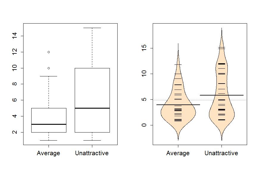
Now the boxplot and beanplots only contain results for the two groups of interest here as seen in Figure 1-6.
> boxplot(Years~Attr,data=MockJury2)
> beanplot(Years~Attr,data=MockJury2,log="",col="bisque",method="jitter")
The two-sample mean techniques you learned in your previous course start with comparing the means the two groups. We can obtain the two means using the mean function or directly obtain the difference in the means using the compareMean function (both require the mosaic package). The compareMean function provides xUnattractive−xAverage where x is the sample mean of observations in the subscripted group. Note that there are two directions to compare the means and this function chooses to take the mean from the second group name alphabetically and subtracts the mean from the first alphabetical group name. It is always good to check the direction of this calculation as having a difference of -1.84 years versus 1.84 years could be important to note.
> mean(Years~Attr,data=MockJury2)
| Average | Unattractive |
| 3.973684 | 5.810811 |
> compareMean(Years ~ Attr, data=MockJury2)
[1] 1.837127