0.1 - Getting started in R
by
This book and access to a computer (PC, Mac, or just computer lab computers on campus) are the only required materials for the course. You will need to download the statistical software package called R and an enhanced interface to R called R-studio (Rstudio, 2014). They are open source and free to download and use (and will always be that way). This means that the skills you learn now can follow you the rest of your life. R is becoming the primary language of statistics and is being adopted across academia, government, and businesses to help manage and learn from the growing volume of data being obtained. Hopefully you will get a sense of some of the power of R this semester.
The next pages will walk you through the process of getting the software downloaded and provide you with an initial experience using R-studio to do things that should look familiar even though the interface will be a new experience. Do not expect to master R quickly - it takes years (sorry!) even if you know all the statistical methods being used. We will try to keep all of your interactions with R code in a similar coding form and that should help your learning how to use R as we move through various methods. Everyone that learns R starts with copying other people's code and then making changes for specific applications - so expect to go back to examples and learn how to modify that code to work for your particular data set. In Chapter 1, we will exploit the power of R to compare quantitative responses from two groups, making some graphical displays, doing hypothesis testing and creating confidence intervals in a couple of different ways.
You will have two downloading activities to complete before you can do anything more than read this book. First, you need to download R. It is the engine that will do all the computing for us, but you will only interact with it once. Go to http://cran.rstudio.com and click on the "Download R for..." button that corresponds to your operating system. Second, you need to download R-studio. It is an enhanced interface that will make interacting with R less frustrating. Go to http://www.rstudio.com/products/rstudio/download/ and select the "installer" for your operating system under the column for "Installers for all platforms". From this point forward, you should only open R-studio; it provides your interface with R. Note that both R and R-studio are updated frequently (up to four times a year) and if you downloaded either more than a few months previously, you should download the up-to-date versions, especially if something you are trying to do is not working. Sometimes code will not work in older versions of R and sometimes old code won't work in new versions of R3.
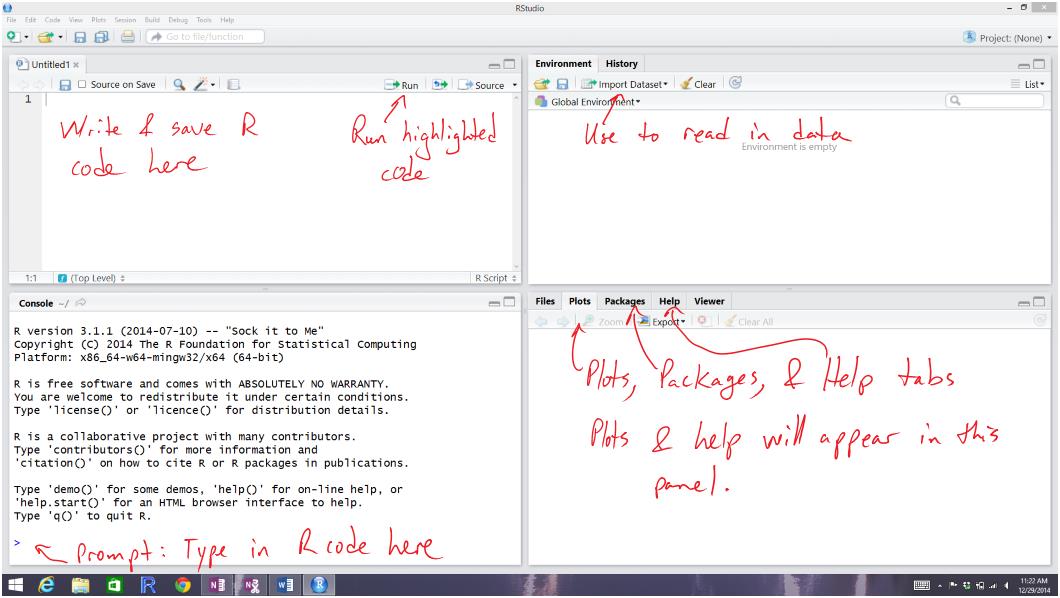
Now we get to complete some basic tasks in R using the R-studio interface. When you open R-studio, you will see a screen like Figure 0-2. The added notes can help you get initially oriented to the software interface. R is command-line software - meaning that most of the time you have to create code and then execute it to get any results. R-studio makes the management and execution of code more efficient than the basic version of R. The lower left panel in R-studio is called the "console" window and is where you can type R code directly into R or where you will see the code you run and (most importantly!) where the results of your executed commands will show up. The most basic interaction with R is available once you get the cursor active at the command prompt ">". The upper left panel is for writing, saving, and running your R code. Once you have code available in this window, the "Run" button will execute the code for the line that your cursor is on or for any text that you have highlighted with your mouse. The "data management" or environment panel is in the upper right, providing information on what data sets have been loaded. It also contains the "Import Dataset" button that makes reading data into R easier. The lower right panel contains information on the "Packages" that are available and is where you will see plots that you make and requests for "Help".
To interact with R, click near the command prompt (>) in the lower left "console" panel, type 3+4 and then hit enter. It should look like this:
> 3+4
[1] 7
You can do more interesting calculations, like finding the mean of the numbers 3, 5, 7, and 8 by adding them up and dividing by 4:
(-3+5+7+8)/4
[1] 4.25
Note that the the parentheses help R to figure out your desired order of operations. If you drop that grouping, you get a very different result:
> -3+5+7+8/4
[1] 11
We could estimate the standard deviation similarly using the formula you might remember from introductory statistics, but that will only work in very limited situations. To use the real power of R this semester, we need to work with data sets that store the observations for our subjects in variables. Basically, we need to store observations in named vectors that contain a list of the observations. To create a vector containing the four numbers and assign it to a variable named variable1, we need to create a vector using the function c which means combine the items that follow if they are inside parentheses and have commas separating the values:
> c(-3,5,7,8)
[1] -3 5 7 8
To get this vector stored in a variable called variable1 we need to use the assignment operator, "<-"(read as "stored as") that assigns in the information on the right into the variable that you are creating.
> variable1 <- c(-3,5,7,8)
In R, the assignment operator, <-, is created by typing a less than symbol (<) followed by a minus sign (-) without a space between them. If you ever want to see what numbers are residing in an object in R, just type its name and hit enter. You can see how that variable contains the same information that was initially generated by c(-3,5,7,8) but is easier to access since we just need the text representing that vector.
> variable1
[1] -3 5 7 8
You can see how that variable contains the same information that was initially generated by c(-3,5,7,8) but is easier to access since we just need the text representing that vector. Now we can use functions such as mean and sd to find the mean and standard deviation of the observations contained in variable1:
> mean(variable1)
[1] 4.25
> sd(variable1)
[1] 4.99166
When dealing with real data, we will often have information about more than one variable. We could enter all observations by hand for each variable but this is prone to error and onerous for all but the smallest data sets. If you are to ever utilize the power of statistics in the evolving data-centered world, data management has to be accomplished in a more sophisticated way. While you can manage data sets quite effectively in R, it is often easiest to start with your data set in something like Microsoft Excel or OpenOffice's Calc. You want to make sure that observations are in the rows and the names of variables are in the columns and that there is no "extra stuff" in the spreadsheet. If you have missing observations, they should be represented with blank cells. The file should be saved as a ".csv" file (stands for comma-separated values although Excel calls it "CSV (Comma Delimited)", which basically strips off some of the junk that Excel adds to the necessary information in the file. Excel will tell you that this is a bad idea, but it actually creates a more stable long-term storage format and one that R can use directly. There will be a few words in the last chapter regarding why we use R in this course instead of Excel or other (commercial) statistical software. We'll wait until we show you some of the cool things that R can do to discuss why we didn't use other software.
With a data set converted to a CSV file, we need to read the data set into R. There are two ways to do this, either using the GUI point-and-click interface in R-studio or modifying the read.csv function to find the file of interest. To practice this, you can download an Excel (.xls) file from https://dl.dropboxusercontent.com/u/77307195/treadmill.xls that contains observations on 31 males that volunteered for a study on methods for measuring fitness (Westfall and Young, 1993). In the spreadsheet, you will find:
| Subject | TreadMillOx | TreadMillMaxPulse | RunTime | RunPulse | RestPulse | BodyWeight | Age |
| 1 | 60.05 | 186 | 8.63 | 170 | 48 | 81.87 | 38 |
| 2 | 59.57 | 172 | 8.17 | 166 | 40 | 68.15 | 42 |
| ... | ... | ... | ... | ... | ... | ... | .... |
| 30 | 39.2 | 172 | 12.88 | 168 | 44 | 91.63 | 54 |
| 31 | 37.39 | 192 | 14.03 | 186 | 56 | 87.66 | 45 |
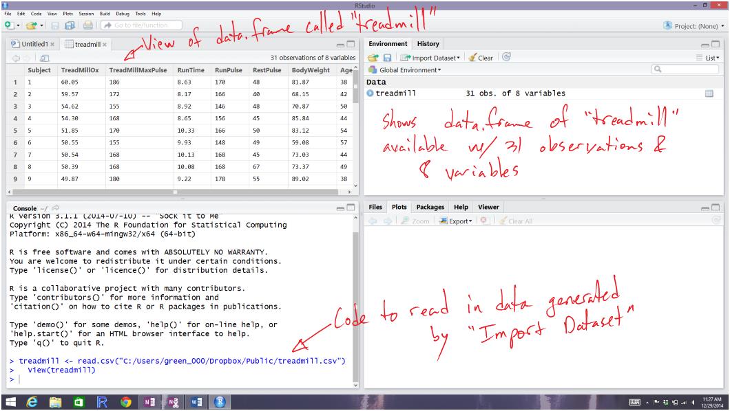
The variables contain information on the subject number (Subject), subjects' treadmill oxygen consumption (TreadMillOx, in ml per kg per minute) and maximum pulse rate (TreadMillMaxPulse, in beats per minute), minutes to run 1.5 miles (Run Time), maximum pulse during 1.5 mile run (RunPulse, in beats per minute), resting pulse rate (RestPulse, beats per minute), Body Weight (BodyWeight, in kg), and Age (in years). Open the file in Excel or equivalent software and then save it as a .csv file in a location you can find. Then go to R-studio and click on Tools, then Import Data Set, then From Text File...4 Find your file and check "Import". R will store the data set as an object named whatever the .csv file was named. You could use another name as well, but it is often easiest just to keep the data set name in R related to the original file. You should see some text appear in the console like in Figure 0-3. The text that is created will look something like the following (depending on the location you stored the file) - if you had stored the file in a drive labeled D:/, it would be:
treadmill <- read.csv("D:/treadmill.csv")
What is put inside the " " will depend on the location of your saved .csv file. A version of the data set in what looks like a spreadsheet will appear in the upper left window due to the second line of code (View(treadmill)). Just directly typing (or using) a line of code like this is actually the other way that we can read in files. If you choose to use this, you need to tell R where to look in your computer to find the data file. read.csv is a function that takes a path as an argument. To use it, specify the path to your data file, put quotes around it, and put it as the input to read.csv(...). For some examples later in the book, you will be able to copy a command like this and read data sets and other code directly from my Dropbox folder using an internet connection.
To verify that you read in the data set correctly, it is good to check its contents. We can view the first and last rows in the data set using the head and tail functions on the data set, which show the following results for the treadmill data. Note that you will sometimes need to resize the console window in R-studio to get all the columns to display in a single row which can be performed by dragging the grey bars that separate the panels.
>head(treadmill)
| Subject | TreadMillOx | TreadMillMaxPulse | RunTime | RunPulse | RestPulse | BodyWeight | Age | |
| 1 | 1 | 60.05 | 186 | 8.63 | 170 | 48 | 81.87 | 38 |
| 2 | 2 | 59.57 | 172 | 8.17 | 166 | 40 | 68.15 | 42 |
| 3 | 3 | 54.62 | 155 | 8.92 | 146 | 48 | 70.87 | 50 |
| 4 | 4 | 54.30 | 168 | 8.65 | 156 | 45 | 85.84 | 44 |
| 5 | 5 | 51.85 | 170 | 10.33 | 166 | 50 | 83.12 | 54 |
| 6 | 6 | 50.55 | 155 | 9.93 | 148 | 49 | 59.08 | 57 |
>tail(treadmill)
| Subject | TreadMillOx | TreadMillMaxPulse | RunTime | RunPulse | RestPulse | BodyWeight | Age | |
| 26 | 26 | 44.61 | 182 | 11.37 | 178 | 62 | 89.47 | 44 |
| 27 | 27 | 40.84 | 172 | 10.95 | 168 | 57 | 69.63 | 51 |
| 28 | 28 | 39.44 | 176 | 13.08 | 174 | 63 | 81.42 | 44 |
| 29 | 29 | 39.41 | 176 | 12.63 | 174 | 58 | 73.37 | 57 |
| 30 | 30 | 39.20 | 172 | 12.88 | 168 | 44 | 91.63 | 54 |
| 31 | 31 | 37.39 | 192 | 14.03 | 186 | 56 | 87.66 | 45 |
While not always required, for many of the analyses, we will tap into a large suite of additional functions available in R packages by "installing" (basically downloading) and then "loading" the packages. There are some packages that we will use frequently, starting with the mosaic package (Pruim, Kaplan, and Horton, 2014). To install a R package, go to the Packages tab in the lower right panel of R-studio. Click on the Install button and then type in the name of the package in the box (here type in mosaic). R-studio will try to auto-complete the package name you are typing which should help you make sure you got it typed correctly. This will be the first of many times that we will mention that R is case sensitive - in other words, Mosaic is different from mosaic in R syntax. You should only need to install each R package once on a given computer. If you ever see a message that R can't find a package, make sure it appears in the list in the Packages tab and if it doesn't, repeat the previous steps to install it.
After installing the package, we need to load it to make it active. We need to go to the command prompt and type (or copy and paste) require(mosaic):
> require(mosaic)
You may see a warning message about versions of the package and versions of R - this is usually something you can ignore. Other warning messages could be more ominous for proceeding but before getting too concerned, there are couple of basic things to check. First, double check that the package is installed. Second, check for typographical errors in your code - especially for mis-spellings or unintended capilization. If you are still having issues, try repeating the installation process or find someone more used to using R to help you. Most computers in computer labs on campus at MSU have R and R-studio installed and provide another venue to use the software if you are having problems5.
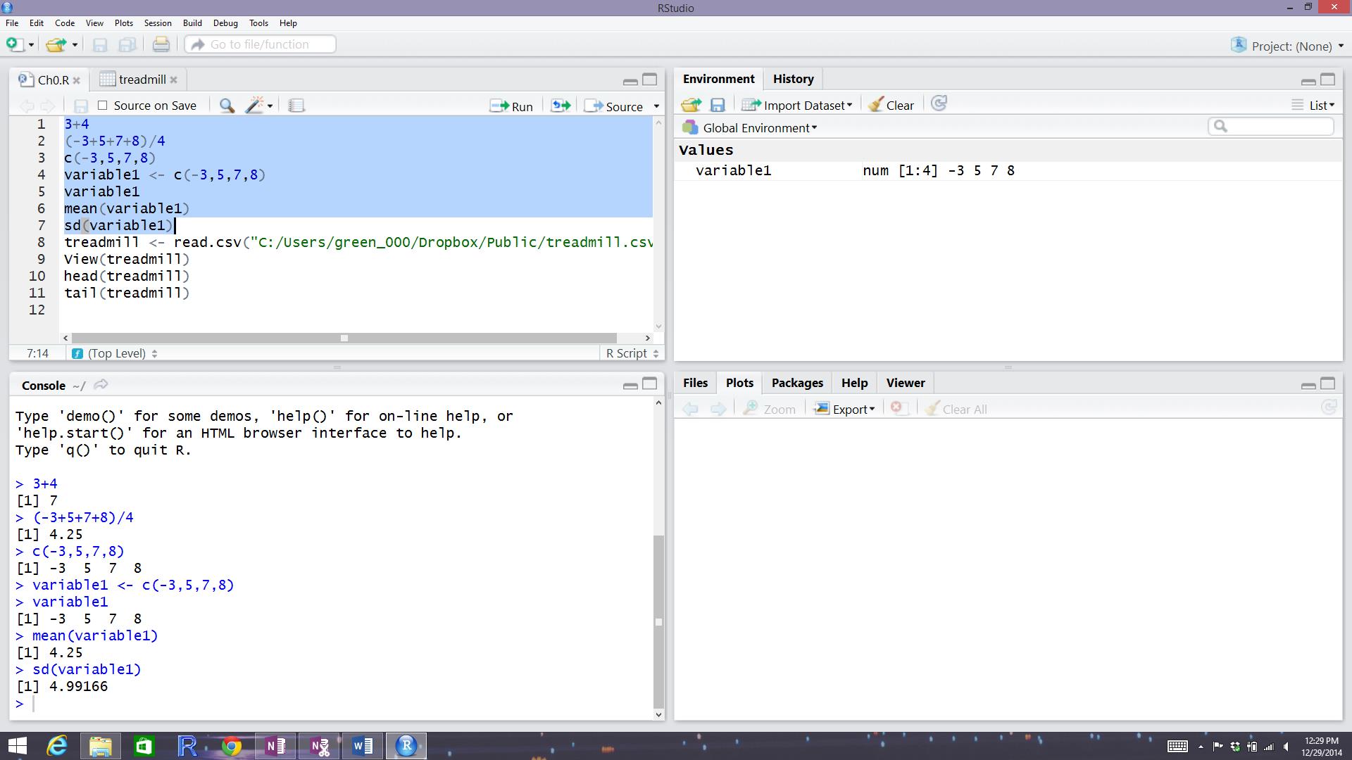
To help you go from basic to intermediate R usage, you will want to learn how to manage and save your R code. The best way to do this is using the upper left panel in R-studio using what are called R-scripts and they have a file extension of .R. To start a new .R file to store your code, click on File, then New File, then R Script. This will create a blank page to enter and edit code - then save the file as MyFileName.R in your preferred location. Saving your code will mean that you can return to where you last were working by simply re-running the saved script file. With code in the script window, you can place the cursor on a line of code or highlight a chunk of code and hit the "Run" button on the upper part of the panel. It will appear in the console with results just like what you got if you typed it after the command prompt. Figure 0-4 shows the screen with the code used in this section in the upper left panel, saved in file called Ch0.R, with the results of highlighting and executing the first section of code using the "Run" button.
3The need to keep the code up-to-date as R continues to evolve is one reason that this book is locally published...
4If you are having trouble getting the file converted and read into R, copy and run the following code: treadmill=read.csv("http://dl.dropboxusercontent.com/u/77307195/treadmill.csv",header=T)
5We highly recommend that you do not wait until the last minute to try to get R code to work for your own assignments. Even experienced R users can sometimes need a little time to find their errors.