0.0 - Overview of methods
by
After an introduction to statistics, a wide array of statistical methods become available. This course re-iterates a variety of themes from the first semester course including the basics of statistical inference and statistical thinking - and it assumes you remember the general framework of ideas from that previous experience. The methods explored focus on assessing (estimating and testing for) relationships between variables - which is where statistics gets really interesting and useful. Early statistical analyses (approximately 100 years ago) were focused on describing a single variable. Your introductory statistics course should have heavily explored methods for summarizing and doing inference in situations with one or two groups of observations. Now, we get to consider more complicated situations - culminating in a set of tools for working with situations with multiple explanatory variables, some of which might be categorical. Throughout the methods, it will be important to retain a focus on how the appropriate statistical analysis depends on the research question and data collection process as well as the types of variables measured.
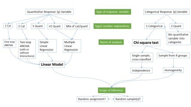
Figure 0-1 frames the topics we will discuss. Taking a broad vision of the methods we will consider, there are basically two scenarios - one when the response is quantitative (meaningful numerical quantity for each case) and one when the response is categorical (divides the cases into groups, placing each case into one and only one category. Examples of quantitative responses we will see later involve suggested jail sentence (in years) and body fat (percentage. Examples of categorical variables include improvement (none, some, or marked) in a clinical trial or whether a student has turned in copied work (never, exam or paper, or both. There are going to be some more nuanced aspects to all of these analyses as the complexity of two trees suggest, but note that near the bottom, each tree converges on a single procedure, using a linear model for quantitative response variables and a Chi-square test for a categorical response. After selecting the appropriate procedure and completing the necessary technical steps to get results for a given data set, the final step involves assessing the scope of inference and types of conclusions that are appropriate based on the design of the study.
The number of analysis techniques is directly proportional to our focus in this class, and we will be spending most of the semester working on methods for quantitative response variables (the left side of Figure 0-1 covered in Chapters 1, 2, 3, 5, 6, and 7) and stepping over to handle the situation with a categorical response variable (right side of Figure 0-1 discussed in Chapter 4). The final chapter contains case studies illustrating all of the methods discussed previously, providing an opportunity to see how finding your way through the paths in Figure 0-1 leads to the appropriate analysis.
The first topics (Chapters 0 and 1) will be more familiar as we start with single and two group situations with a quantitative response. In your previous statistics course, you should have seen methods for estimating and quantifying uncertainty for differences in two groups. Once we have briefly reviewed these methods and introduced the statistical software that we will use throughout the course, we will consider the first truly new material in Chapter 2. It involves the situation where there are more than 2 groups to compare with a quantitative response - this is what we call the One-Way ANOVA situation. It generalizes the 2 independent sample test to handle situations where more than 2 groups are being studied. When we learn this method, we will begin discussing model assumptions and methods for assessing those assumptions that will be present in every analysis involving a quantitative response. The Two-Way ANOVA (Chapter 3) considers situations with two categorical explanatory variables and a quantitative response. To make this somewhat concrete, suppose we are interested in assessing differences in biomass based on the amount of fertilizer applied (none, low, or high) and species of plant (two types). Here, biomass is a quantitative response variable and there are two categorical explanatory variables, fertilizer, with 3 levels, and species, with two levels. In this material, we introduce the idea of an interaction between the two explanatory variables: the relationship between one categorical variable and the mean of the response changes depending on the levels of the other categorical variable. For example, extra fertilizer might enhance the growth of one species and hinder the growth of another so fertilizer has different impacts based on the level of species. Given that this interaction may or may not be present, we will consider two versions of the model in Two-Way ANOVAs, what are called the additive (no interaction) and the interaction models.
Following the methods for two categorical variables and a quantitative response, we explore a method for analyzing data where the response is categorical, called the Chi-square test in Chapter 4. This most closely matches the One-Way ANOVA situation with a single categorical explanatory variable, except now the response variable is categorical. For example, we will assess whether taking a drug (vs taking a placebo1) has an effect2 on the type of improvement the subjects demonstrate. There are two different scenarios for study design that impact the analysis technique and hypotheses tested in Chapter 4. If the explanatory variable reflects the group that subjects were obtained from, either through randomization of the treatment level to the subjects or by taking samples from separate populations, this is called a Chi-square Homogeneity test. It is also possible to analyze data using the same Chi-square test that was generated by taking a single sample from a population and then obtaining information on the levels of the explanatory variable for each subject. We will analyze these results using what is called a Chi-square Independence test.
If the predictor and response variables are both quantitative, we start with correlation and simple linear regression models (Chapters 5 and 6) - things you should have seen, at least to some degree, previously. If there is more than one quantitative explanatory variable, then we say that we are doing multiple linear regression (Chapter 7) - the "multiple" part of the name reflects that there will be more than one explanatory variable. If the situation suggests the use of a mix of categorical and quantitative predictor variables, then we also call the models multiple linear regression models. In the situation with one categorical predictor and one quantitative predictor, we revisit the idea of an interaction. It allows us to consider situations where the estimated relationship between a quantitative predictor and the mean response varies among different levels of the categorical variable.
At the end of the course, you should be able to identify, perform using the statistical software R (R Core Team, 2014), and interpret the results from each of these methods. There is a lot to learn, but many of the tools for using R and interpreting results of the analyses accumulate during the semester. If you work hard to understand the initial methods, it will help you when the methods get much more complicated. All of the methods you will learn require you to carefully consider how the data were collected, how that pertains to the population of interest, and how that impacts inferences that can be made. The scope of inference is our shorthand term for remembering to think about two aspects of the study - random assignment and random sampling. One aspect of this assessment is to decide if the explanatory variable was randomly assigned to study units (allowing for causal inferences if differences are detected) or not (so no causal statements are possible). The other aspect concerns random sampling: If the data were obtained using a random sampling mechanism, then our inferences can be safely extended to the population that the sample was taken from. However, if we have random sample, our inference can only apply to the sample collected. You will often think you are done with your analysis when you get some numbers from R, but need to remember to think about the potential conclusions you can make based on the source of the data set you are analyzing. By the end of this course, you should have some basic R skills and abilities to create basic ANOVA and Regression models, as well as Chi-squared testing situations. Together, this should prepare you for future STAT courses or for other situations where you are expected to be able to do the calculations and effectively communicate interpretations for the methods discussed in this course.
1A placebo is a treatment level designed to mimic the potentially efficacious level(s) but that can have no actual effect. The placebo effect is the effect that thinking that an effective treatment was received has on subjects.
2We will reserve the term "effect" for situations where we could potentially infer causal impacts on the response of the explanatory variable which occurs in situations where the levels of the explanatory variable are randomly assigned to the subjects.