2.1 - Linear model for One-Way ANOVA (cell-means and reference-coding)
by
We introduced the statistical model γij = μj + εij in Chapter 1 for the situation with j = 1 or 2 to denote a situation where there were two groups and, for the alternative model, the means differed. Now we have three groups and the previous model can be extended to this new situation by allowing j to be 1, 2, or 3. Now that we have more than two groups, we need to admit that what we were doing in Chapter 1 was actually fitting what is called a linear model. The linear model assumes that the responses follow a normal distribution with the linear model defining the mean, all observations have the same variance, and the parameters for the mean in the model enter linearly. This last condition is hard to explain at this level of material - it is sufficient to know that there models where the parameters enter the model nonlinearly and that they are beyond the scope of this course. The result of this constraint is that we will be able to use the same general modeling framework for the rest of the course.
As in Chapter 1, we have a null hypothesis that defines a situation (and model) where all the groups have the same mean. Specifically, the null hypothesis in the general situation with J groups (J≥2) is to have all the true group means equal,
H0: μ1 =... = μJ.
This defines a model where all the groups have the same mean that we can define in terms of a single mean, μ, for the ith observation from the jth group as γij = μ + εij. This is not the model that most researchers want to characterize their study as it implies no difference in the groups. There is more caution required to specify the alternative hypothesis with more than two groups. The alternative hypothesis needs to be the logical negation of this null hypothesis of all groups having equal means; to make the null hypothesis false, we only need one group to differ but more than one group could differ from the others. Essentially, there are many ways to "violate" the null hypothesis so we choose some delicate wording for the alternative hypothesis when there are more than 2 groups. Specifically, we state the alternative as
HA: Not all μj are equal
or, in words, at least one of the true means differs among the J groups. You will be attracted to trying to say that all means are different in the alternative but we do not put this strict a requirement in place to reject the null hypothesis. The alternative model allows all the true group means to differ but does require that they differ with
γij = μj + εij.
This linear model states that the response for the ith observation in the jth group, γij, is modeled with a group j (j=1,...,J) population mean, μj, and a random error for each subject in each group, εij, that we assume follows a normal distribution and that all the random errors have the same variance, σ2. We can write the assumption about the random errors, often called the normality assumption, as εij~N(0,σ2). There is a second way to write out this model that will allow extensions to more complex models discussed below, so we need a name for this version of the model. The model writtern in terms of the μj's is called the cell means model and is the easier version of this model to understand.
One of the reasons we learned about beanplots is that it helps us visually consider all the aspects of this model. In the right panel of Figure 2-1, we can see the wider, bold horizontal lines that provide the estimated group means. The bigger the differences, the more likely we are to find evidence against the null hypothesis. You can also see the null model on the plot that assumes all the groups have the same as displayed in the dashed horizontal line at 4.7 years (the R code below shows the overall mean of Years is 4.7). While the hypotheses focus on the means, the model also contains assumptions about the distribution of the responses - specifically that the distributions are normal and all have the groups have the same variability. As discussed previously, it appears that the distributions are right skewed and the variability might not be the same for all the groups. The boxplot provides the information about the skew and variability but since it doesn't display the means it is not directly related to the linear model and hypotheses we are considering.
> mean(MockJury$Years)
[1] 4.692982
There is a second way to write out the One-Way ANOVA model that will allow extensions to more complex models in Chapter 3. The other parameterization (way of writing out or defining) of the model is called the reference-coded model since it writes out the model in terms of a baseline group and deviations from that baseline or reference level. The reference-coded model for the ith subject in the jth group is yij = α + τj + εij where α (alpha) is the true mean for the baseline group (first alphabetically) and the τj (tau j) are the deviations from the baseline group for group j. The deviation for the baseline group, τ1, is always set to 0 so there are really just deviations for groups 2 through J. The equivalence between the two models can be seen by considering the mean for the first, second, and Jth groups in both models:
| Cell means: | Reference-coded | |
| Group 1: | μ1 | α |
| Group 2: | μ2 | α + τ2 |
| ... | ... | ... |
| Group J: | μJ | α + τJ |
The hypotheses for the reference-coded model are similar to those in the cell-means coding except that they are defined in terms of the deviations, τj. The null hypothesis is that there is no deviation from the baseline for any group - that all the τj's =0,
H0: τ2 =... = τJ = 0.
The alternative hypothesis is that at least one of the deviations is not 0,
HA: Not all τj equal 0.
You are welcome to use either version unless we instruct you to use a particular version in this chapter but we have to use the reference-coding in subsequent chapters. The next task is to learn how to use R's linear model (lm) function to get estimates of the parameters in each model, but first a review of these new ideas:
Cell-means version:
• H0: μ1 =... = μJ HA: Not all μj equal
• Null hypothesis in words: No difference in the true means between the groups.
• Null model: yij = μ + εij
• Alternative hypothesis in words: At least one of the true means differs between the groups.
• Alternative model: yij = μj + εij
Reference-coded version:• H0: τ2 =... = τJ = 0 HA: Not all τj equal 0
• Null hypothesis in words: No deviation of the true mean for any groups from the baseline group.
• Null model: yij = α + εij
• Alternative hypothesis in words: At least one of the true deviations is different from 0 or that at least one group has a different true mean than the baseline group.
• Alternative model: yij = α + τj + εij
In order to estimate the models discussed above, the lm function will be used. If you look closely in the code for the rest of the semester, any model for a quantitative response will use this function, suggesting a common threads in the most commonly used statistical models. The lm function continues to use the same format as previous functions, lm(Y~X,data=datasetname). It ends up that this code will give you the reference-coded version of the model by default. We want to start with the cell-means version of the model, so we have to add a "-1" to the formula interface to tell R that we want to the cell-means coding. Generally, this looks like lm(Y~X-1,data=datasetname) and you will find a row of output for each group. It will contain columns for an estimate (Estimate), standard error (Std. Error), t-value (t value), and p-value (Pr(>|t|)). We'll learn to use all of the output in the following material, but for now we will just focus on the estimates of the parameters that the function provides that we put in bold.
> lm1 <- lm(Years~Attr-1,data=MockJuryR)
> summary(lm1)
Coefficients:
| Estimate | Std.Error | t value | Pr(>|t|) | ||
| AttrBeautiful | 4.3333 | 0.5730 | 7.563 | 1.23e-11 | *** |
| AttrAverage | 3.9737 | 0.5805 | 6.845 | 4.41e-10 | *** |
| AttrUnattractive | 5.8108 | 0.5883 | 9.878 | < 2e-16 | *** |
In general, we denote estimated parameters with a hat over the parameter of interest to show that it is an estimate. For the true mean of group j, μj, we estimate it with μ̂j, which is just the sample mean for group j, xj. The model suggests an estimate for each observation that we denote as ŷij that we will also call a fitted value based on the model being considered. The three estimates are bolded in the previous output, with a different estimate produced for all observations in the same group. R tries to help you to sort out which row of output corresponds to which group by appending the group name with the variable name. Here, the variable name was Attr and the first group alphabetically was Beautiful, so R provides a row labeled AttrBeautiful with an estimate of 4.3333. The sample means from the three groups can be seen to directly match those results.
> mean(Years~Attr,data=MockJuryR)
| Beautiful | Average | Unattractive |
| 4.333333 | 3.973684 | 5.810811 |
The reference-coded version of the same model is more complicated but ends up giving the same results once we understand what it is doing. Here is the model summary:
> lm2 <- lm(Years~Attr,data=MockJuryR)
> summary(lm2)
Coefficients:
| Estimate | Std. Error | t value | Pr(>|t|) | ||
| (Intercept) | 4.3333 | 0.5730 | 7.563 | 1.23e-11 | *** |
| AttrAverage | -0.3596 | 0.8157 | -0.441 | 0.6601 | |
| AttrUnattractive | 1.4775 | 0.8212 | 1.799 | 0.0747 | . |
Residual standard error: 3.578 on 111 degrees of freedom
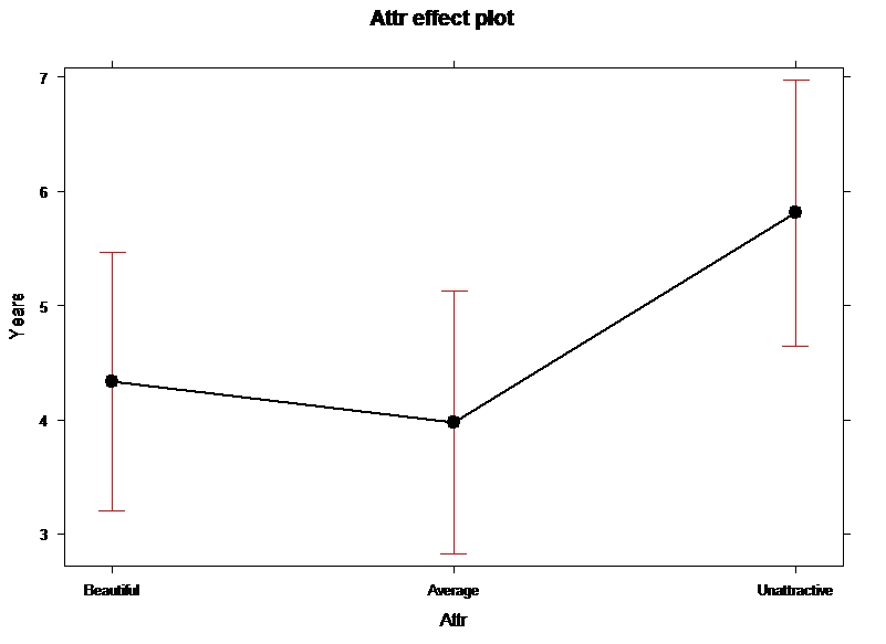
Multiple R-squared: 0.04754, Adjusted R-squared: 0.03038 F-statistic: 2.77 on 2 and 111 DF, p-value: 0.067 Remember that this is the standard version of the linear model so it will be something that gets used repeatedly this semester. The estimated model coefficients are α̂ = 4.333 years, τ̂2 =-0.3596 years, and τ̂3 =1.4775 years where group 1 is Beautiful, 2 is Average, and 3 is Unattractive. The way you can figure out the baseline group (group 1 is Beautiful here) is to see which category label is not present in the output. The baseline level is typically the first group label alphabetically, but you should always check this. Based on these definitions, there are interpretations available for each coefficient. For α̂ = 4.333 years, this is an estimate of the mean sentencing time for the Beautiful group. τ̂2 =-0.3596 years is the deviation of the Average group's mean from the Beautiful groups mean (specifically, it is 0.36 years lower). Finally, τ̂3 =1.4775 years tells us that the Unattractive group mean sentencing time is 1.48 years higher than the Beautiful group mean sentencing time. These interpretations lead directly to reconstructing the estimated means for each group by combining the baseline and pertinent deviations as shown in Table 2-1. We can also visualize the results of our linear models using what are called term or effect plots (from the effects package; Fox, 2003) as displayed in Figure 2-2 (we don't want to use "effect" unless we have random assignment in the study design so we will mainly call these term plots). These plots take an estimated model and show you its estimates along with 95% confidence intervals generated by the linear model, which will be especially useful for some of the more complicated models encountered later in the semester. To make this plot, you need to install and load the effects package and then use plot(allEffects(...)) functions together on the lm object called lm2 generated above. You can find the correspondence between the displayed means and the estimates that were constructed in Table 2-1. > require(effects) > plot(allEffects(lm2)) In order to assess evidence for having different means for the groups, we will compare either of the previous models (cell-means or reference-coded) to a null model based on the null hypothesis (H0: μ1 =... = μJ) which implies a model of yij = μ + εij in the cell-means version where μ is a common mean for all the observations. We will call this the mean-only model since it is boring and only has a single mean in it. In the reference-coding version of the model, we have a null hypothesis that H0: τ2 =... = τJ = 0, so the "mean-only" model is yij = α + εij with α having the same definition as μ for the cell means model - it forces a common estimate for every group. The mean-only model is also an example of a reduced model where we set some coefficients in the model to 0 and get a simpler model. Simple can be good as it is easy to interpret, but having a model for J groups that suggests no difference in the groups is not a very exciting result in most, but not all, situations. In order for R to provide results for the mean-only model, we remove the grouping variable, Attr, from the model formula and just include a "1". The (Intercept) row of the output provides the estimate for either model when we assume that the mean is the same for all groups: > lm3 <- lm(Years~1,data=MockJuryR) > summary(lm3) Coefficients: Residual standard error: 3.634 on 113 degrees of freedom This model provides an estimate of the common mean for all observations of 4.693 = μ̂=α̂ years. This value also is the dashed, horizontal line in the beanplot in Figure 2-1.
Group Formula Estimates Beautiful α̂ 4.3333 years Average α̂ + τ̂2 4.3333-0.3596=3.974 years Unattractive α̂ + τ̂3 4.3333+1.4775=5.811 years
Estimate Std. Error t value Pr(>|t|) (Intercept) 4.6930 0.3404 13.79 <2e-16 ***